Benchmark - Hakuna Ma-data: Identify Wildlife on the Serengeti with AI for Earth¶

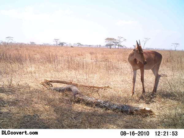
Welcome to the benchmark solution tutorial for our new competition in partnership with AI for Earth! In this computer-vision competition, you are tasked with identifying animal species in camera trap footage. The training data consists of over 2.5 million sequences of images collected using camera traps placed in the Serengeti region of Africa. The sequences are one-hot-labeled for 53 different species groups, or as empty. For each sequence (which may be multiple images), you will generate a submission that consists of probabilities for each possible class.

But the fun doesn't stop there! In this competition, you will not be submitting a csv of predictions. Instead, you will submit the code that performs inference on the test data, and we will execute that code in the cloud to generate and score your submission.

In this benchmark, we'll walk through a first-pass approach to loading, understanding, and preparing the data. We'll use an out-of-the-box transfer learning approach to train a Keras model on a subset of the training data. Then we'll explain how to package up your model and submit a file capable of running in our cloud-based execution environment. With all these pipes connected, you'll be ready to hit the ground running.

We've got a large territory to cover, so let's get started!

Data Exploration¶

Our training set consists of 10 "seasons" of footage. We can get information about each seson's sequences and labels using the training metadata, which provides links between image flenames and sequences, as well as the training labels, which tell us what's in a given sequence.

You can download the metadata as well as the actual image data here. Keep in mind, this is a very large training set, so make sure you have a storage solution. The complete set of images for all 10 seasons is nearly 5 TB! But the image data is split by season, so you can download image files one season at a time. For this benchmark, we're only going to work with a couple of seasons.

Let's load the metadata and look at what we have.

Number of images in the train set.

That's a lot of images! However, each image is associated to a sequence. And our predictions will be at the sequence level.

A sequence is an ordered series, in this case of camera trap images ordered in time. When the camera trap is triggered, it often takes more than one image, yielding a an image sequence. In the data, each sequence has a seq_id, which is the index for the labels. The order of images in a given sequence can be inferred from the last four digits in the filename.

Since our predictions are made at the sequence level, this means that there is one label for any given sequence. Imagine that lion walks by and triggers the camera trap, which takes 4 pictures. If the lion keeps walking, they may only appear in the first three pictures in the sequence and be out of frame by the time the 4th image is taken. Despite the 4th frame being empty of any lion, that sequence of 4 images would still be labeled as lion.

Let's confirm that each label in train_labels corresponds to a unique seq_id.

We have different seasons in the training set, and different numbers of images per season. We can see which season an image belongs to by looking at the first few characters of the sequence ID.

Keep in mind that the test set comes from seasons not represented in the training set. So our model needs to generalize to seasons it hasn't seen before.

As we can see, location values are not unique between seasons. So while our model will need to generalize across seasons, it might get to "revisit" the same location from season to season.

Below we see that the number of images we have for each sequence varies, but by far most sequences have between 1 and 3 images in them.

For this benchmark, we're going to simplify the problem by taking only the first image from each sequence. The justifying assumption here is that the period of time immediately after a camera trap is first triggered is the most likely time to see an animal in frame. However, this may not always be the case and ultimately you'll probably want to give your model as much information as you can by using more images per sequence.

Now, let's look at the labels. Each sequence label is a one-hot-encoded row vector with a 1 in the coloumn corresponding to a species that is present, and a 0 otherwise. Each row corresponds to a unique sequence ID.

Though most sequences have only one animal in them, it is possible to mutliple animals in a single sequence.

Notice below that not only is empty a category, but it's the most dominant category––by far! This is because, as useful as camera traps are, they tend to register many false positives. For example, they are often triggered by wind blowing plant life around, or fluctuations of heat and light in the surrounding area.

Now that we have a sense of what the data means, let's get access to the images themselves!

Dealing With Large Amounts of Data¶

Since there are millions of high-quality images, unzipping all the data takes a long time. We recommend starting your model development with a single season or two of data while the rest of the data downloads. In this benchmark, we'll work with seasons 1 and 3.

Add Full Image Path to the Data¶

Our local data is mounted under the /databig/raw directory in folders that match the name of the zipfile.

We'll convert the file_name column to a Path object with the full path to our data.

Before we get into the weeds of modeling, let's take a quick break to look at some of animals in this data!

A particular animal that catches our eye is the ... zorilla? Let's check it out.

Cute. What else?

Wow! Ok maybe just one more...

Looks like someone wants a belly rub!

Ok, we really should get back to work.

Splitting the Data in a Reasonable Way¶

As we mentioned above, we know the test set for this comeptition involves seasons we have no access to. For training, however, we do have access to metadata and downloads for 10 seasons. We should set aside some portion of these seasons to validate our model during development. That way we are less likely to see misleading validation results due to overfitting one or more seasons.

In this benchmark, we're going to use season 1 for training, and season 3 for validation. You'll likely want to use multiple seasons for training and validation in your model.

Using A Data Generator¶

We have way too many images to load into memory. We're going to need a data generator that can stream data to our model. Recall that to simplify our first pass solution we aren't using the whole sequence, just the first image in each sequence. That allows us to treat the problem as a standard image classification probablem, which is fine for this benchmark but you'll probably want to generalize the approach to include all the information from the sequences!

Because we've reduced the problem to a simpler one, we can use the standard ImageDataGenerator packaged with Keras.

One of the many cool things about this generator is that it has a method called .flow_from_dataframe, allowing us to get batches of images using a dataframe that includes paths to the files and the labels. First we'll need to join the file paths the the labels.

Next we instantiate the generators, one for training and one for validation data. Once our model is compiled, we'll use the .fit_generator method instead of .fit to train, passing in the data generators instead of the traditional x_train, y_train, x_val, y_val. The generators will then give the model one batch at a time so that we can worry less about overloading the memory with too many awesome camera trap shots!

...Like this one!

Anyways, since we have so many blanks we're going to lazily balance our training set by dropping most of them and avoid predicting blank for everything. This is a start, but you'll probably want to delop a better approach for avoiding an overfit model.

That looks at least like a 2 class problem. Note we didn't change the validation set's class balance, so we should be able to get a fair sense of how our model generalizes.

Let's use this data to set up the generators.

Ok! We're now ready to create the model.

Creating the model¶

We want to keep the model reatlively simple for a first pass, adding complexity only after we have tested a basic approach. As mentioned above, because we only consider the first image of each sequence, we don't need to (more like we don't get to) consider any of the exicting complications that arise from sequence modeling. Instead, we can treat the problem as a standard image classification problem.

We're going to use a fixed feature extractor approach to transfer learning. This just means that we're going to use a pretrained model but freeze all the weights inside of the model and swap out the classifier at the top of the model. In tensorflow.keras this can be done in just a few lines as follows:

1. Import a pretrained model without its classification layer
2. Turn off the pretrained trainable attributes for faster training
3. Collect the outputs of the pretrained model and pass them along to additional layers, or the classifier.
4. Add a classification layer that matches our problem

Note: This modeling approach could be extended to handle sequences but you'll probably have to write your own generator in addition to using, for example, tensorflow.keras.layers.TimeDistributed layers, but that exercise is left to the reader!

There are lots of pretrained models to choose from. We're going to choose NasNet, simply because it demonstrates state-of-the-art performance on the ImageNet dataset. Although the top-performing model is NASNetLarge, we're going to speed things up a bit by using the smaller NASNetMobile.

We'll compile the model using a standard optimization with respect to categorical crossentropy loss. For metrics, in addition to loss we'll consider two versions of top-K accuracy. The K just means "the correct prediction was in the top K most-probable classes." We're used to top-1 accuracy, but in image problems, top-5 is typically considered as well. Top-5 accuracy can help us see if the right labels are "bubbling up" towards higher probability.

Time to train! We'll train on about 13,000 examples and validate on half of that.

Make Submission¶

Submissions for this competition work in a different way than usual in that the inference code is actually executed to generate the score. This means we'll need to

• save our model
• factor our data loading and preprocessing code
• write inference code to create a submission
• package everything up and upload to the DrivenData + Microsoft execution environment in the cloud!

The key part of the submission process is the main.py file which loads the model and weights, performs inference on the test data, and saves out predictions to submission.csv. You can see this benchmark's example main.py file here.

Let's walk through the process. Below we will

1. Put all files needed to generate a submission in a folder called inference/. Our main.py script will live at the root level. The main.py script will be run in our cloud-based execution environment, which expects a submission.csv to be generated at the root level (next to main.py) when inference is complete.

2. To support the inference process, we'll use a subdirectory of inference/ called assets/ to store

   • our trained model weights
   • the submission format, used to check the validitiy of our submission
   • the test metadata, used by our data generator to fetch batches of data to perform inference

3. We'll zip the contents of the inference directory (not the directory itself) into a file called submission.zip.

4. When we upload submission.zip, the file will be unzipped and main.py will be run in a gpu-enabled Docker container with many data science libraries installed. The runtime environment can be seen here.

First, let's make the inference directory and its assets subdirectory.

Now let's save our model!

We also need to make sure the script has access to the submission format and test metadata, so we copy test_metadata.csv and submission_format.csv into the assets folder as well.

Below we will paste the entirety of our main.py script. You may want to study the script and comments closely. A few things to notice

• DATA. During execution, our data lives in the cloud mounted at inference/data/. We'll need to use the test_metadata.csv and the cloud data path to construct the full paths to be used by our generator
• WORKERS. Our model.predict_generator method uses the workers parameter to use multiple cores and threads for data loading and inference generation. This improves inference speed by more than a factor of 10 compared to using single core default settings. You'll need to utilize parallelism or other efficiency measures to meet the execution time requirement whihc requires your inference process to take no more than TIME hours.
• PREPROCESSING. Notice that we import our preprocessing function tensorflow.keras.applications.nasnet.preprocess_input. This is crucial for performance consistence with training so make sure your preprocessing code is available to main.py!

Let's take a look at the contents we'll be zipping up, then you can study the main.py script.

Great! Read over main.py below and read on to check out the results of our submission.

Our main.py submission script¶

Now we'll zip everything up, submit it, and get our score!

Upload submission¶

Alright! We're ready to submit!

Our submission takes about 20 minutes to execute. Once it's complete, we can see our score id around 0.05! Awesome!

Hopefully this benchmark helps you understand the submission process for this exciting new type of DrivenData competition.

We can't wait to see what you come up with! Happy importing!

Oh, and don't forget: