Huzzah. Our new competition predicting fog water collection from weather data is up! Let's put on our DATA SCIENCE HATS and get to work.
TL;DR version
Here's what we're doing right now: looking at the microclimate measurements as independent snapshots in time as predictors of the outcome variable. You can grab the notebook on Github and follow along at home.
Cool stuff we're not doing (but that the winners will undoubtedly explore)
Here's what we're NOT doing right now:
- Using macro-climate weather data at different levels of sampling to add information and reduce variance.
- Any form of time series modeling, like, at all.
- Incorporating more complex models of the underlying system we wish to model. And by complex here we mean "vaguely realistic."
Here's a new term for y'all courtesy of the DrivenData team:
Somebody throw it on Urban Dictionary — let's make fetch happen. Okay, time to load up the tools of the trade.
%matplotlib inline
from __future__ import print_function

from matplotlib import pyplot as plt
import seaborn as sns

import numpy as np
import pandas as pd
Loading the data
For this benchmark, we are only going to use microclimate data.
microclimate_train = pd.read_csv(
    "data/eaa4fe4a-b85f-4088-85ee-42cabad25c81.csv", index_col=0, parse_dates=[0]
)

microclimate_test = pd.read_csv(
    "data/fb38df29-e4b7-4331-862c-869fac984cfa.csv", index_col=0, parse_dates=[0]
)

labels = pd.read_csv(
    "data/a0f785bc-e8c7-4253-8e8a-8a1cd0441f73.csv", index_col=0, parse_dates=[0]
)

submission_format = pd.read_csv(
    "data/submission_format.csv", index_col=0, parse_dates=[0]
)
Looking at the training data (we are given labels for these)
First of all, let's just "walk around" this data a bit, and use the common summary functions to get a better idea for what it looks like.
microclimate_train.shape
microclimate_train.describe()
microclimate_train.tail()
microclimate_train.isnull().sum(axis=0)
Here's the big takeway: we will have to deal with some missing values.
Looking at the test data (we will be predicting labels for these rows)
microclimate_test.shape
microclimate_test.describe()
microclimate_train.isnull().sum(axis=0)
So again, we will definitely need to pay attention to missing values and figure out smart ways to deal with that. File under #datascientistproblems.
Let's also plot all the data points in the training and test data to get a sense for how the data set is split:
fig, axs = plt.subplots(
    nrows=microclimate_train.shape[1], ncols=1, sharex=True, figsize=(16, 18)
)

columns = microclimate_train.columns
for i, ax in list(enumerate(axs)):
    col = columns[i]
    ax.plot_date(microclimate_train.index, microclimate_train[col], ms=1.5, label="train")
    ax.plot_date(
        microclimate_test.index, microclimate_test[col], ms=1.5, color="r", label="test"
    )
    ax.set_ylabel(col)

    if i == 0:
        ax.legend(loc="upper right", markerscale=10, fontsize="xx-large")

This isn't your grandpa's random train/test split
Here's another fun insight: this problem has a time component and in the real world we are trying to predict the future. That is, we're trying to figure out the upcoming yield based on current weather. For those of us concerned about overfitting (hint: all of us), we will need to think hard about our modeling assumptions.
So, things that we could do but probably shouldn't:
- Imputing missing values using all of the data.
- Treating every data point as if it stands alone and is independent from other points in time.
- Drawing on weather that hasn't happened yet to inform our current predictions.
But this is a benchmark and we're not all about rules on this blog. Watch us break every single one of these cautionary warnings below! (That's why they call it a benchmark. (Actually that statement doesn't make sense, we don't know why it's called a benchmark. (HOLY MOLY, TOO MANY PARENTHESES #inception #common-lisp)))
Looking at relationships between inputs and yield
print("train", microclimate_train.shape)
print("labels", labels.shape)
microclimate_train.columns.tolist()
wanted_cols = [
    "percip_mm",
    "humidity",
    "temp",
    "leafwet450_min",
    "leafwet_lwscnt",
    "wind_ms",
]
wanted = microclimate_train[wanted_cols].copy().dropna()
wanted["yield"] = labels["yield"]

sns.pairplot(wanted, diag_kind="kde")
plt.show()

We can see some relationships starting to emerge here, but maybe not as directly correlated with yield as we may have hoped.
Splitting the data
Quick nomenclature check: we are training our model on the competition's training data, but we still need to use some cross validation techniques to avoid overfitting the heck out of the data.
We'll go ahead and split up the competition training set into its own training and test sets for our modeling purposes here.
from sklearn.cross_validation import train_test_split

X_train, X_test, y_train, y_test = train_test_split(
    microclimate_train, labels.values.ravel(), test_size=0.3
)
Building a model pipeline
Here's a scikit-learn pipeline which will handle a couple tasks for us in a well defined, repeatable way:
- Setting up an imputer to replace missing data.
- Try out some dimensionality reduction with PCA.
- Train the world's most naive random forest classifier.
And we'll GRID SEARCH ALL THE THINGS, because, hey, why not, right???!1
from sklearn.pipeline import Pipeline
from sklearn.decomposition import PCA
from sklearn.preprocessing import Imputer
from sklearn.grid_search import GridSearchCV
from sklearn.ensemble import RandomForestRegressor

steps = [("imputer", Imputer()), ("pca", PCA()), ("rf", RandomForestRegressor())]
pipe = Pipeline(steps)

# create the grid search
params = {
    "pca__n_components": range(2, X_train.shape[1]),
    "imputer__strategy": ["mean", "median", "most_frequent"],
    "rf__n_estimators": [5, 10, 20],
}
estimator = GridSearchCV(pipe, param_grid=params, n_jobs=-1, verbose=1)
estimator.fit(X_train, y_train.ravel())
estimator.best_params_
Examine performance
The competition uses root mean squared error as the metric, so let's see how we do on that front.
from sklearn.metrics import mean_squared_error

y_hat = estimator.predict(X_test)
rmse = np.sqrt(mean_squared_error(y_test, y_hat))
rmse
We can also plot our actuals against our predicted values and see if there's a trend.
fig, ax = plt.subplots(figsize=(8, 8))
plt.scatter(y_test, y_hat)

plt.xlabel("actual", fontsize=20)
plt.ylabel("predicted", fontsize=20)
plt.plot(np.linspace(0, 35), np.linspace(0, 35), label="$y=x$")

plt.xlim(0, 35)
plt.ylim(0, 35)
plt.legend(loc="upper left", fontsize=20)
plt.show()

Let's look at the residuals by themselves:
fig, ax = plt.subplots(figsize=(16, 4))
err = y_test - y_hat

ax.plot_date(X_test.index, err, c="r", ms=3)
ax.set_title("residuals on test data (each)", fontsize=20)
ax.set_ylabel("error")

plt.show()

And also look at the distribution of residuals.
fig, ax = plt.subplots(figsize=(16, 4))
plt.hist(err, bins=20, normed=True)
plt.title("residuals on test data (distribution)", fontsize=20)
plt.xlim(-20, 20)
plt.show()

So we have our predictions in hand, and we have some idea of the error (although in practice this number only makes sense compared to other submissions — yet another great reason to give people a benchmark even with a very naive model!)
Time to make this into a submission.
What should our submission look like?
So we know we need to predict the labels from the training inputs we were given, but let's just double check how it's supposed to look.
!head data/submission_format.csv
submission_format.head()
submission_format.dtypes
submission_format.shape
microclimate_test.shape
We'll do a quick and dirty mitigation by making sure the test data we pass into our pipline has an input row for each and every expected row in the submission format, even if they are all NaNs.
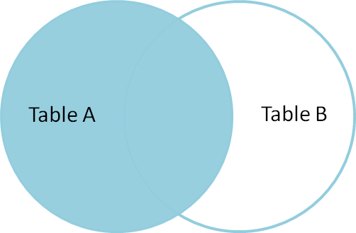
An easy way to get the right index for our purposes is a left outer join, where the "left hand" table is our submission format and the "right hand table" is the microclimate data we have. The left join will link every row that has an identical index in both sets, but will fill the rows in microclimate that do not exist as NaNs.
Here's a helpful figure from Jeff Atwood's helpful post on the topic:
test = submission_format.join(microclimate_test, how="left")  # left join onto the format
test = test[microclimate_test.columns]  # now just subset back down to the input columns

assert (test.index == submission_format.index).all()
Making our submission
We'll make predictions and fill in the yield column with actual outputs from our model:
submission_format["yield"] = estimator.predict(test)
Now we'll write it out to a file:
submission_format.to_csv("first_submission.csv")
And we can submit it to the competition and see what we end up with:

Ouch. The overfitting police have come to lay down the law. Note how we ended up scoring much more poorly on the withheld evaluation data than on our own withheld test set. That's a clear indication we overfit the data.
But the gauntlet has been thrown down. Will you step up to beat this ... pettifogging model?