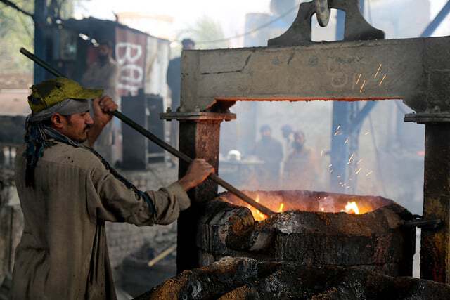
Measuring poverty is hard, but The World Bank plans to end extreme poverty by 2030 – and they need your help! Poverty levels are often estimated at the country level by extrapolating the results of surveys taken on a subset of the population at the household or individual level.
The surveys are incredibly informative, but they are also incredibly long. A typical poverty survey has hundreds of questions, ranging from region-specific questions to questions about the last time a participant bought bread. In order to track progress towards its goal, The World Bank needs the most efficient survey possible. That's where you come in.
 For more information, explore this recent World Bank report on ending the cycle of poverty.
In our brand new competition, we're asking you to predict poverty at the household level by building a great classification model. The strongest poverty predictors could be used by statisticians at The World Bank to design new, shorter, equally informative surveys. With these improvements, The World Bank can more easily track progress towards their ambitious and inspiring goal.
In this post, we'll walk through a very simple first pass model for poverty prediction from survey data, showing you how to load the data, make some predictions, and then submit those predictions to the competition.
To get started, we summon the tools of the trade.
%matplotlib inline

import os

import numpy as np
import pandas as pd

import matplotlib.pyplot as plt

# data directory
DATA_DIR = os.path.join("..", "data", "processed")
Loading the Data
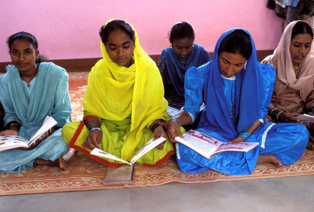
 Check out this research focused on children and the effort to end extreme poverty.
On the data download page, we provide a couple of datasets to get started:
- Household-level survey data: This is obfuscated data from surveys conducted by The World Bank, focusing on household-level statistics. The data come from three different countries, and are separated into different files for convenience.
- Individual-level survey data: This is obfuscated data from related surveys conducted by The World Bank, only these focus on individual-level statistics. The set of interviewees and countries involved are the same as the household data, as indicated by shared
idindices, but this data includes detailed (obfuscated) information about household members. - Submission format: This gives us the filenames and columns of our submission prediction, filled with all
0.5as a baseline.
In classic benchmark fashion, we're going to keep this analysis short, sweet, and simple. As such, we're not going to use any of the individual-level data that's included with the competition. Even without individual-level data, we have a lot of files to deal with. It's probably worth it to store our paths in an easily-accessible dictionary:
data_paths = {
    "A": {
        "train": os.path.join(DATA_DIR, "A", "A_hhold_train.csv"),
        "test": os.path.join(DATA_DIR, "A", "A_hhold_test.csv"),
    },
    "B": {
        "train": os.path.join(DATA_DIR, "B", "B_hhold_train.csv"),
        "test": os.path.join(DATA_DIR, "B", "B_hhold_test.csv"),
    },
    "C": {
        "train": os.path.join(DATA_DIR, "C", "C_hhold_train.csv"),
        "test": os.path.join(DATA_DIR, "C", "C_hhold_test.csv"),
    },
}
# load training data
a_train = pd.read_csv(data_paths["A"]["train"], index_col="id")
b_train = pd.read_csv(data_paths["B"]["train"], index_col="id")
c_train = pd.read_csv(data_paths["C"]["train"], index_col="id")
As usual, let's take a quick look at the head.
a_train.head()
b_train.head()
c_train.head()
The first thing to notice is that each country's surveys have wildly different numbers of columns, so we'll plan on training separate models for each country and combining our predictions for submission at the end.
Poverty Distributions
Let's take a look at the class distributions for each country. In classification tasks, it's crucial to know the balance of class labels!
a_train.poor.value_counts().plot.bar(title="Number of Poor for country A")

b_train.poor.value_counts().plot.bar(title="Number of Poor for country B")

c_train.poor.value_counts().plot.bar(title="Number of Poor for country C")

Country A is well-balanced, but countries B and C are quite unbalanced. This could definitely impact the confidence of our predictor. But solving that problem is up to you – it's outside the scope of this humble benchmark.
We expect most of the data types here to be the dreaded object type, but let's make sure.
a_train.info()
b_train.info()
c_train.info()
Sure enough, the bool types are our labels--the poor column--then there are a few numeric types with the rest being object. We'll need to convert the object columns to categorical variables before training anything.
Pre-process the Data
We're going to do some simple pre-processing here. Standardizing the data and converting the object types to categoricals should get us pretty far. Let's write a couple of simple functions to help this effort.
# Standardize features
def standardize(df, numeric_only=True):
    numeric = df.select_dtypes(include=["int64", "float64"])

    # subtracy mean and divide by std
    df[numeric.columns] = (numeric - numeric.mean()) / numeric.std()

    return df


def pre_process_data(df, enforce_cols=None):
    print("Input shape:\t{}".format(df.shape))

    df = standardize(df)
    print("After standardization {}".format(df.shape))

    # create dummy variables for categoricals
    df = pd.get_dummies(df)
    print("After converting categoricals:\t{}".format(df.shape))

    # match test set and training set columns
    if enforce_cols is not None:
        to_drop = np.setdiff1d(df.columns, enforce_cols)
        to_add = np.setdiff1d(enforce_cols, df.columns)

        df.drop(to_drop, axis=1, inplace=True)
        df = df.assign(**{c: 0 for c in to_add})

    df.fillna(0, inplace=True)

    return df
Time to convert these surveys!
print("Country A")
aX_train = pre_process_data(a_train.drop("poor", axis=1))
ay_train = np.ravel(a_train.poor)

print("\nCountry B")
bX_train = pre_process_data(b_train.drop("poor", axis=1))
by_train = np.ravel(b_train.poor)

print("\nCountry C")
cX_train = pre_process_data(c_train.drop("poor", axis=1))
cy_train = np.ravel(c_train.poor)
The data is probably looking pretty different now. Let's take a peek at country A.
aX_train.head()
Oh yeah, now that looks like the kind of matrix scikit-learn wants to process!
The Error Metric - MeanLogLoss
The error metric for this competition is our old friend, log loss ... with a twist. Since we're predicting for three countries, our overall score is going to be the mean of the log losses for each country. However, the countries labels are conditionally independent, so in practice we should be able to train three independent models and combine their predictions for submission.
See the competition submission page for more info on the metric!
Build the Model
As mentioned above, we're keeping this benchmark short, sweet, and simple. So where do we turn when looking for a great out-of-the-box model? If you answered "Random Forests!" then we may just be two trees of the same ensemble. No? Then perhaps we're... splitting on the same node? At any rate, random forests are often a good model to try first, especially when we have numeric and categorical variables in our feature space.
Random Forest
In scikit-learn, it almost couldn't be easier to grow a random forest with a few lines of code.
from sklearn.ensemble import RandomForestClassifier


def train_model(features, labels, **kwargs):
    # instantiate model
    model = RandomForestClassifier(n_estimators=50, random_state=0)

    # train model
    model.fit(features, labels)

    # get a (not-very-useful) sense of performance
    accuracy = model.score(features, labels)
    print(f"In-sample accuracy: {accuracy:0.2%}")

    return model
 Another classic from xkcd.
That's it as far model building is concerned. Let's grow some trees!
model_a = train_model(aX_train, ay_train)
model_b = train_model(bX_train, by_train)
model_c = train_model(cX_train, cy_train)
Time to Predict and Submit
Remember, accuracy is not a very informative metric, especially when dealing with imbalanced classes. Furthermore, accuracy is not the metric for this competition!
The above scores suggest little more than an overfit training set. But it's confidence that counts – we'll need to use the .predict_proba() method to generate our submissions. Let's load up the test data, process it, and see what we get.
# load test data
a_test = pd.read_csv(data_paths["A"]["test"], index_col="id")
b_test = pd.read_csv(data_paths["B"]["test"], index_col="id")
c_test = pd.read_csv(data_paths["C"]["test"], index_col="id")
# process the test data
a_test = pre_process_data(a_test, enforce_cols=aX_train.columns)
b_test = pre_process_data(b_test, enforce_cols=bX_train.columns)
c_test = pre_process_data(c_test, enforce_cols=cX_train.columns)
Note that we're taking a very simple approach to filling missing values, as well as enforcing column consistency after converting to categoricals. (See the preprocessing function again to see what enforce_cols actually does.)
Make Predictions
To return the confidence probabilities that the submission format requires, we need to call the predict_proba() method on our models.
a_preds = model_a.predict_proba(a_test)
b_preds = model_b.predict_proba(b_test)
c_preds = model_c.predict_proba(c_test)
That was easy enough. Time to format the predictions and send them on their way.
Save Submission
We'll write a simple function that converts the predictions a DataFrame and adds a column for the correct country code.
def make_country_sub(preds, test_feat, country):
    # make sure we code the country correctly
    country_codes = ["A", "B", "C"]

    # get just the poor probabilities
    country_sub = pd.DataFrame(
        data=preds[:, 1],  # proba p=1
        columns=["poor"],
        index=test_feat.index,
    )

    # add the country code for joining later
    country_sub["country"] = country
    return country_sub[["country", "poor"]]
# convert preds to data frames
a_sub = make_country_sub(a_preds, a_test, "A")
b_sub = make_country_sub(b_preds, b_test, "B")
c_sub = make_country_sub(c_preds, c_test, "C")
Finally, it's time to combine our predictions and save for submission!
submission = pd.concat([a_sub, b_sub, c_sub])
How about one last look at the fruits of or hard work...
submission.head()
submission.tail()
Looks good, let's save and send'er off!
submission.to_csv("submission.csv")
Submit to Leaderboard

Woohoo! It's a start! And that's exactly what we intend with these benchmarks. We're sure you'll be able to top this model in no time, and we can't wait to see what you come up with.
 Visit The World Bank's site to learn more about how poverty is measured.