How to Use an LSTM for Timeseries and the Cold-start Problem
Forecasting the energy consumption of a building can play a pivotal role in the operations efficiency of the building. Facility managers, utility companies, and comissioning projects use consumption forecasts to design and implement energy-saving policies that optimize building performance and reduce negative environmental impact.

Typically, the best forecasting algortihms use a lot of historical information about the building they're forecasting for––think past consumption trends, past sensor measurements, past building usage––to compute the forecasts. This requirement presents a big challenge: how can we make accurate predictions for new buildings, which don't have a long consumption history?
This is sometimes described as a "cold start" problem, where we need to make accurate predictions off of little to no initial data. Is it possible to create an accurate forecast wihtout much consumption history? That's where you come in!
In our brand new competition, we're asking you to accurately forecast building energy consumption from the beginning of the building instrumentation life. Given only one day to two weeks of consumption history per building, your task to use this "cold start" data to accurately forecast consumption. Some forecasts will ask for hourly consumption predictions, while others will ask for daily or even weekly projections.
In this post, we'll walk through a simple model for predicting energy consumption over different time horizons using varying amounts of "cold start" consumption data. We'll show you how to load the data, train a model to make some predictions, and then submit those predictions to the competition.
To get started, we import some standard data science libraries for loading, manipulating, and visualizing the data.
%matplotlib inline

# plotting
import matplotlib as mpl

mpl.style.use("ggplot")
import matplotlib.pyplot as plt

# math and data manipulation
import numpy as np
import pandas as pd

# to handle paths
from pathlib import Path

# set random seeds
from numpy.random import seed
from tensorflow import set_random_seed

RANDOM_SEED = 2018
seed(RANDOM_SEED)
set_random_seed(RANDOM_SEED)
Loading the Data
On the data download page, we provide everything you need to get started:
consumption_train.csv- Historical series that can be used as training data.cold_start_test.csv- Cold start lead-in periods for the series that appear in the submission format.meta.csv- Information about the series that are available to competitors.submission_format.csv- This is the format for submssions to the competition. Your submissions must match the columns and indices exactly.
Training Data
The main dataset we'll be using in this benchmark is consumption_train.csv. Since this is meant to be a simple first pass, we won't be using the meta features about the buildings, or even the temperature measurements that are provided in consumption_train.csv. It's up to you to take advantage of all the information!
data_path = Path("..", "data", "final", "public")
consumption_train = pd.read_csv(
    data_path / "consumption_train.csv", index_col=0, parse_dates=["timestamp"]
)
consumption_train.head()
Each series_id has an associated time series of consumption and temperature data. For a given series, the measurements are provided at hourly time-steps. In other words, every row of consumption_train represents an hour of data from series_id. Each unique series_id in consumption_train has four weeks, or 28 days, worth of hourly data.
Let's figure out how many series we have, and how much training data that corresponds to.
def describe_training_data(train_df):
    num_training_series = train_df.series_id.nunique()
    num_training_days = num_training_series * 28
    num_training_hours = num_training_days * 24
    assert num_training_hours == train_df.shape[0]

    desc = (
        f"There are {num_training_series} training "
        f"series totaling {num_training_days} days "
        f"({num_training_hours} hours) of consumption data."
    )

    print(desc)


describe_training_data(consumption_train)
That's a lot of data! In order speed up development and facilitate rapid prototyping, let's reduce the training set. Since all of the training series are the same length, we'll uniformly sample a subset of series. The size of our resulting reduced data will be controlled by frac_series_to_use.
# choose subset of series for training
frac_series_to_use = 0.01

rng = np.random.RandomState(seed=RANDOM_SEED)
series_ids = consumption_train.series_id.unique()
series_mask = rng.binomial(1, frac_series_to_use, size=series_ids.shape).astype(bool)

training_series = series_ids[series_mask]

# reduce training data to series subset
consumption_train = consumption_train[consumption_train.series_id.isin(training_series)]

# describe the reduced set
describe_training_data(consumption_train)
That will speed things up a bit!
Test Data
The cold start data is provided in cold_start_test.csv. This data is what is provided for each new series before the window that we need to predict. There is a different amount of cold-start data provided for different series, and our model needs to work well whether we are given 1 day or 14.
cold_start_test = pd.read_csv(
    data_path / "cold_start_test.csv", index_col=0, parse_dates=["timestamp"]
)
cold_start_test.head()
The predictions windows are obtained from the submission format prediction_window column.
submission_format = pd.read_csv(
    data_path / "submission_format.csv", index_col="pred_id", parse_dates=["timestamp"]
)
submission_format.head()
Let's take a closer look at these time series.
Explore the Data
As mentioned above, the task in this challege is to utilize "cold start" consumption data to generate consumption forecasts for various prediction windows. Each series_id in the test set asks for one (and only one) of three prediction windows:
- hourly - predict consumption each hour for a day (24 predictions)
- daily - predict consumption each day for a week (7 predictions)
- weekly - predict consumption each week for two weeks (2 predictions)
The prediction window types are pretty evenly distributed across the series_ids
# confirm that every series asks for only one type of prediction
assert all(1 == submission_format.groupby("series_id").prediction_window.nunique())

# use the first() prediction window value from a series_id so as not to overcount
submission_format.groupby("series_id").prediction_window.first().value_counts()
For each series_id in the test set, the amount of hourly cold start data you are provided is never less than one day (24 consecutive consumption measurements) and can be as much as two weeks (336 consecutive consumption measurements). Cold start data only comes in full-day chunks. In other words, some series may have 3, 4, ..., 14 days worth of cold start data, but no series have 3.5, 4.1, ..., 13.9, or any other partial-day's worth of cold start data.
Since each timestep represents and hour, we can visually confirm the above claim with a simple bar plot counting the number of days in each test series.
ax = (
    cold_start_test.groupby("series_id")
    .count()
    .timestamp.divide(24)
    .value_counts()
    .sort_index()
    .plot.bar()
)
ax.set_xlabel("Days in Cold Start Data")
ax.set_ylabel("Number of Test Series")
plt.show()
Some series may provide little cold start data and ask for a long (weekly) forecast, while others may provide many days of cold start data and ask for a short (hourly) forecast. Let's take a look at how these scenarios are distributed in the test set.
First, for convenience, we'll add prediction_window to the test data.
# add prediction_window to the test data
pred_windows = submission_format[["series_id", "prediction_window"]].drop_duplicates()
cold_start_test = cold_start_test.merge(pred_windows, on="series_id")

num_cold_start_days_provided = (
    cold_start_test.groupby("series_id").prediction_window.value_counts().divide(24)
)

num_cold_start_days_provided.head()
Now we'll plot the distribution of prediction_window for each unique length of cold start data in the test set.
def _count_cold_start_days(subdf):
    """Get the number of times a certain cold-start period
    appears in the data.
    """
    return (
        subdf.series_id.value_counts()
        .divide(24)  # hours to days
        .value_counts()
    )


cold_start_occurrence = cold_start_test.groupby("prediction_window").apply(
    _count_cold_start_days
)

cold_start_occurrence.head()
ax = cold_start_occurrence.unstack(0).plot.bar(figsize=(10, 6), rot=0)

ax.set_xlabel("Number of Cold-start Days")
ax.set_ylabel("Number of Series in Dataset");
It looks like the various combinations are all represented, with a couple of combinations being more or less represented. However, there does not seem to be any advantage to building this into our algorithm.
Of course, you aren't only provided with cold start data. The main training set, consumption_train has many series, each with 4 weeks worth of hourly data. To gain a sense of what the cold start prediction asks of you, let's look at a few examples of how the cold start data leads up to the prediction window.
# visualize the cold start and prediction windows
num_to_plot = 40

fig, ax = plt.subplots(figsize=(45, 15))

cold_start_map = {"hourly": 1, "daily": 7, "weekly": 14}

rng = np.random.RandomState(seed=5425)
series_to_plot = rng.choice(cold_start_test.series_id.unique(), num_to_plot)

for i, series_id in enumerate(series_to_plot):
    # get relevant information about the test series from coldstart data
    series_data = cold_start_test[cold_start_test.series_id == series_id]
    start_cold = series_data.timestamp.min()
    start_preds = series_data.timestamp.max()

    # get prediction stop from submission format
    stop_preds = submission_format[
        submission_format.series_id == series_id
    ].timestamp.max()

    # plot the cold start and prediction window relative sizes
    ax.plot([start_cold, start_preds], [i, i], c="#6496e5", linewidth=num_to_plot / 3)
    ax.plot([start_preds, stop_preds], [i, i], c="#e25522", linewidth=num_to_plot / 3)

# the y tick labels don't mean anything so turn them off
ax.set_yticks([])
plt.tick_params(labelsize=35)
plt.legend(["Cold Start (1-14 Days)", "Prediction Window"], fontsize=30)

plt.title(f"{num_to_plot} Series Cold Starts And Their Prediction Windows", fontsize=50);
Hopefully this gives you a sense of how you can use the training data to simulate all of the possible cold start scenarios you'll enounter in the test set. For example, at one extreme the 4 weeks can be split into 2 weeks of simulated cold start, followed by two weeks worth of hourly consumption that you can use to create a validation set (by summing the consumption for each week, leading to 2 weekly predictions). At the other extreme, you can take the first day of consumption data from a 4 week long series as cold start and forecast the next 2 weeks in the same way.
Using the series consumption_train, all cold start windows from 1 to 14 days can be created, with a minimum of 14 more days that can be used to create validation sets.
Finally, let's take a look at the consumption patterns in a few series to see that they're 4 weeks.
# plot a few consumption patterns
series_to_plot = rng.choice(consumption_train.series_id.unique(), 3)

for ser_id in series_to_plot:
    ser_data = consumption_train[consumption_train.series_id == ser_id]
    ax = ser_data.plot(
        x="timestamp", y="consumption", title=f"series_id {int(ser_id)}", legend=False
    )
    plt.ylabel("consumption (watt-hours)")
    plt.show()
We can see that all of the series in the training data (even though we just selected a few at the top of this notebook) have the same length.
(
    consumption_train.groupby("series_id")
    .timestamp.apply(lambda x: x.max() - x.min())
    .value_counts()
)
The Error Metric - Normalized Mean Absolute Error
The performance metric is a normalized version of mean absolute error. The normalization coefficient $c_{i}$ for the $i^{\text{th}}$ prediction is composed of a ratio of two numbers,
$$ c_i = \frac{w_i}{m_i} $$where $w_i$ is a weight that makes weekly (24 / 2), daily (24 / 7), and hourly (24 / 24) predictions equally important, and $m_i$ is the true mean consumption over the prediction window under consideration (this mean is unknown to competitors). Multiplying predictions by this coefficient makes each prediction equally important and puts hourly, daily, and weekly predictions on the same scale.
Given the above definition, the metric $NMAE$ is
$$ NMAE = \frac{1}{N} \sum_{i=1}^{N}|\hat{y_i} - y_i|c_i $$- $N$ - The total number of consumption predictions submitted, including all hourly, daily, and weekly predictions
- $\hat{y}$ - The predicted consumption value
- $y$ - The actual consumption value
- $c$ - The normalization coefficient that weights and scales each prediction to have the same impact on the metric
Note The coefficients $c$ are not available to competitors for the test set because the true mean consumptions for the $i^{\text{th}}$ prediction window, $m_i$ are not available to competitors. For the training set, competitors can calculate $m_i$ when creating their own validation sets.
Build the Model
This challenge asks you to take variable length time series as inputs (the cold start data) and map them to variable length time series as outputs (the prediction window). Putting our jargon hats on, we can call this a variable length input variable length output sequence to sequence time series regression problem. While there are many approaches to time series problems, we're going to use a straightforward strategy that relies on a small Long Short Term Memory (LSTM) neural network.
Long Short Term Memory (LSTM) Network
Long Short Term Memory (LSTM) networks can learn patterns over long sequences and do not neccessarily rely on a pre-specified window of lagged observation as input. Further, their internal states can be built up to include information about cold start data before making any number of forecast predictions we ask for. This means that a single LSTM model can handle all prediction horizons in the data. Our overall approach will be to train the network on 4 week series, then use the cold start data to prime the netowrk's internal state for forecasting, and then forecast.
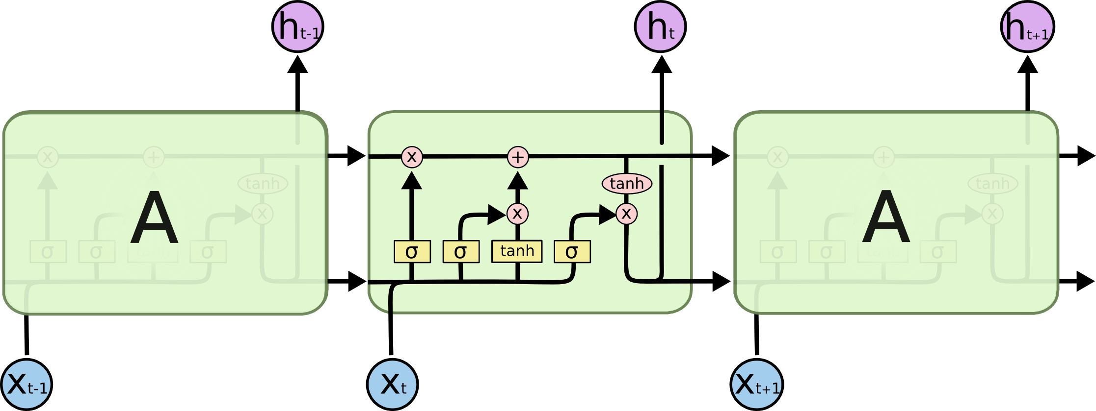
Below we'll go through what's needed to set up a one-step forecast model using the Keras LSTM layer. First, let's consider how to process the data below.
Preparing the data
Appropriately preprocessing data is always important. To prepare our data for modeling with an LSTM let's consider a few standard approaches.
Scaling
Due to their dependence on backpropogation, LSTM networks behave best when the data is within the scale of the activation function used (tanh by default in LSTM, domain $(-1, 1)$). Scikit Learn's MinMaxScaler is sufficient for this task, since it allows us to specify a range and invert transformations.
Stationary
Often in timeseries problems, you want to ensure that your data is stationary, and make it so if it isn't (for example using differencing). That is beyond the scope of this benchmark!
Converting Timeseries to Supervised
We'll use a standard lagged variable approach to convert the timeseries problem to a supervised learning problem, where given features $X$ and labels $y$ the model learns a mapping between them. In this case, the features are our lagged series and the label is the orginal series. This process can be used with any model, but the advantage here is that we can use a stateful LSTM that learns dependencies between each timestep in the data.
def create_lagged_features(df, lag=1):
    if not type(df) == pd.DataFrame:
        df = pd.DataFrame(df, columns=["consumption"])

    def _rename_lag(ser, j):
        ser.name = ser.name + f"_{j}"
        return ser

    # add a column lagged by `i` steps
    for i in range(1, lag + 1):
        df = df.join(df.consumption.shift(i).pipe(_rename_lag, i))

    df.dropna(inplace=True)
    return df


# example series
test_series = consumption_train[consumption_train.series_id == 100283]
create_lagged_features(test_series.consumption, lag=3).head()
Function to Prepare Training Data for Model
Before each series is processed, we'll need to convert it to a supervised learning problem, then scale the data. Let's create a function, prepare_training_data that we can call on each sample in our training loop.
from sklearn.preprocessing import MinMaxScaler


def prepare_training_data(consumption_series, lag):
    """Converts a series of consumption data into a
    lagged, scaled sample.
    """
    # scale training data
    scaler = MinMaxScaler(feature_range=(-1, 1))
    consumption_vals = scaler.fit_transform(consumption_series.values.reshape(-1, 1))

    # convert consumption series to lagged features
    consumption_lagged = create_lagged_features(consumption_vals, lag=lag)

    # X, y format taking the first column (original time series) to be the y
    X = consumption_lagged.drop("consumption", axis=1).values
    y = consumption_lagged.consumption.values

    # keras expects 3 dimensional X
    X = X.reshape(X.shape[0], 1, X.shape[1])

    return X, y, scaler


_X, _y, scaler = prepare_training_data(test_series.consumption, 5)
print(_X.shape)
print(_y.shape)
print(scaler)
Make Model
Now we're ready to build the model. A single LSTM cell followed by a dense layer for regression is a simple base model that we can start with. Let's import Keras objects with a Tensorflow backend. (If you're new to Tensorflow and Keras, see installation instructions here).
# modeling
import keras
from keras.models import Sequential
from keras.layers import LSTM, Dense

# progress bar
from tqdm import tqdm
As usual with Keras, getting from imports to a simple custom model be done in just a few lines. Next we'll instantiate a Keras Sequential configuration and add to it a single recurrent cell followed by a dense layer to output regressed values. We'll also keep the number of neurons in the LSTM cell (this is just the dimensionality of the LSTM output) and the number of passes through the data small.
Note the importance of setting
stateful=Truebelow. This allows the LSTM to learn the patterns within a batch (the lagged series data). Otherwise the state would be reset after each time step, but we want the model to develop states that depend on every timestep we show it.
# lag of 24 to simulate smallest cold start window. Our series
# will be converted to a num_timesteps x lag size matrix
lag = 24

# model parameters
num_neurons = 24
batch_size = 1  # this forces the lstm to step through each time-step one at a time
batch_input_shape = (batch_size, 1, lag)

# instantiate a sequential model
model = Sequential()

# add LSTM layer - stateful MUST be true here in
# order to learn the patterns within a series
model.add(LSTM(units=num_neurons, batch_input_shape=batch_input_shape, stateful=True))

# followed by a dense layer with a single output for regression
model.add(Dense(1))

# compile
model.compile(loss="mean_absolute_error", optimizer="adam")
Fit Model
Now for the fun part! Above we showed that the series in consumption_train could be used to simulate all sorts of cold start types. Here we're just going to fit each 4 week series using a 24 hour lag, so that ideally the model learns at least patterns over a single day.
To train, we pass through the consumption data, grouped by series_id. For each series, we first prepare_training_data, then fit using that data, resetting the state only after each row of the series has been seen. In this way, each lagged timeseries is learned by the network before the state is reset and the next series is passed in.
To keep this example quick, we're only going to make a single pass through the data. An easy way to improve this benchmark is to simply change num_passes_through_data below (to a much larger number).
%%time
num_training_series = consumption_train.series_id.nunique()
num_passes_through_data = 3

for i in tqdm(
    range(num_passes_through_data),
    total=num_passes_through_data,
    desc="Learning Consumption Trends - Epoch",
):
    # reset the LSTM state for training on each series
    for ser_id, ser_data in consumption_train.groupby("series_id"):
        # prepare the data
        X, y, scaler = prepare_training_data(ser_data.consumption, lag)

        # fit the model: note that we don't shuffle batches (it would ruin the sequence)
        # and that we reset states only after an entire X has been fit, instead of after
        # each (size 1) batch, as is the case when stateful=False
        model.fit(X, y, epochs=1, batch_size=batch_size, verbose=0, shuffle=False)
        model.reset_states()
Time to Predict and Submit
To generate our submission, we'll loop over submission format grouping by series_id as above. Within each iteration, we'll need to
- prepare the cold start data
- generate the forecast
To generate the forecast, we'll
- build up the internal state using the prepared cold start data
- predict all hours in the prediction window
- aggregate the forecast appropriately for the submission
To simplify the prediction loop, let's write a couple of functions to accomplish the above tasks.
Function to Generate Forecast
The forecast will start by using the cold start data to build up the state. Then the final cold start prediction will be used to initialize the rest of the forecast. the output of the previous prediction will be used as input to the next predcition. Finally, we just need to invert the scaling at the end to get back to normal consumption values.
def generate_hourly_forecast(num_pred_hours, consumption, model, scaler, lag):
    """Uses last hour's prediction to generate next for num_pred_hours,
    initialized by most recent cold start prediction. Inverts scale of
    predictions before return.
    """
    # allocate prediction frame
    preds_scaled = np.zeros(num_pred_hours)

    # initial X is last lag values from the cold start
    X = scaler.transform(consumption.values.reshape(-1, 1))[-lag:]

    # forecast
    for i in range(num_pred_hours):
        # predict scaled value for next time step
        yhat = model.predict(X.reshape(1, 1, lag), batch_size=1)[0][0]
        preds_scaled[i] = yhat

        # update X to be latest data plus prediction
        X = pd.Series(X.ravel()).shift(-1).fillna(yhat).values

    # revert scale back to original range
    hourly_preds = scaler.inverse_transform(preds_scaled.reshape(-1, 1)).ravel()
    return hourly_preds
Before we start forecasting, let's make a copy of the submission format for our submission.
# copy submission format and fill in values
my_submission = submission_format.copy()
Make Predictions: Forecast the Cold Start Data
Our forecast essentially uses the two above functions. The only other step is that some predictions need to be aggregated, since our forecasts all start as hourly. The dictionary pred_window_to_num_preds specifies the aggregation, then Numpy's split function can be used to aggregate the right amount.
Note: Because this basic approach generates a forecast for every hour of the prediction window, it takes a bit of time (10-15 minutes) to generate all predictions.
%%time
pred_window_to_num_preds = {"hourly": 24, "daily": 7, "weekly": 2}
pred_window_to_num_pred_hours = {"hourly": 24, "daily": 7 * 24, "weekly": 2 * 7 * 24}

num_test_series = my_submission.series_id.nunique()

model.reset_states()

for ser_id, pred_df in tqdm(
    my_submission.groupby("series_id"),
    total=num_test_series,
    desc="Forecasting from Cold Start Data",
):
    # get info about this series' prediction window
    pred_window = pred_df.prediction_window.unique()[0]
    num_preds = pred_window_to_num_preds[pred_window]
    num_pred_hours = pred_window_to_num_pred_hours[pred_window]

    # prepare cold start data
    series_data = cold_start_test[cold_start_test.series_id == ser_id].consumption
    cold_X, cold_y, scaler = prepare_training_data(series_data, lag)

    # fine tune our lstm model to this site using cold start data
    model.fit(cold_X, cold_y, epochs=1, batch_size=batch_size, verbose=0, shuffle=False)

    # make hourly forecasts for duration of pred window
    preds = generate_hourly_forecast(num_pred_hours, series_data, model, scaler, lag)

    # reduce by taking sum over each sub window in pred window
    reduced_preds = [pred.sum() for pred in np.split(preds, num_preds)]

    # store result in submission DataFrame
    ser_id_mask = my_submission.series_id == ser_id
    my_submission.loc[ser_id_mask, "consumption"] = reduced_preds
Check Scale of Prediction
As a quick check, we expect the mean hourly prediction to be smaller than the daily prediction, which is in turn smaller than the weekly prediction.
my_submission[my_submission.prediction_window == "hourly"].consumption.describe()
my_submission[my_submission.prediction_window == "daily"].consumption.describe()
my_submission[my_submission.prediction_window == "weekly"].consumption.describe()
Did the network learn to forecast reasonable looking patterns?
# plot samples
sample_ser = (
    my_submission[my_submission.prediction_window == "hourly"]
    .series_id.sample()
    .values[0]
)

(
    my_submission[my_submission.series_id == sample_ser].plot(
        x="timestamp", y="consumption", title=sample_ser, rot=90
    )
)
Save Submission
my_submission.head(5)
save_path = Path("..", "data", "submissions")
save_path.mkdir(exist_ok=True, parents=True)

my_submission.to_csv(save_path / "my_submmission.csv", index_label="pred_id")
!head ../data/submissions/my_submmission.csv
Submit to the Leaderboard

Woohoo! It's a start! And that's exactly what we intend with these benchmarks. We're sure you'll be able to top this model in no time, and we can't wait to see what you come up with. Happy importing!


