Accurate seasonal water supply forecasts are crucial for effective water resources management in the Western United States. This region faces dry conditions and high demand for water, and these forecasts are essential for making informed decisions. They guide everything from water supply management and flood control to hydropower generation and environmental objectives.
Yet, hydrological modeling is a complex task that depends on natural processes marked by inherent uncertainties, such as antecedent streamflow, snowpack accumulation, soil moisture dynamics, and rainfall patterns. To maximize the utility of these forecasts, it's essential to provide not just accurate predictions, but also comprehensive ranges of values that effectively convey the inherent uncertainties in the predictions.
In the Water Supply Forecast Rodeo, participants were tasked with developing accurate water supply forecast models for 26 sites across the Western United States. This was a probabilistic forecasting task—models needed to predict not just a point estimate for the water supply volume but also uncertainty bounds. Specifically, participants were asked to predict the 0.10, 0.50, and 0.90 quantiles of the water supply at 26 sites in the Western United States.

Challenge Structure
The Water Supply Forecast Rodeo has been one of DrivenData's longest-running and most complex challenges. It was held over multiple stages designed to support solvers in iterative and rigorous model development. 540 participants from 79 different countries participated over the course of the challenge, and over 2,500 forecast submissions were made.
Solvers first developed their solutions on historical data in the Hindcast Stage, which concluded in spring 2024. A separate blog post describes the results and winners of the Hindcast Stage, all of whom won prizes in subsequent phases. This blog post presents the winners of all remaining stages:
- Forecast Stage—where models made near-real-time forecasts for the 2024 forecast season.
- Final Stage Overall Prizes—where models were rigorously evaluated with cross-validation and model reports were judged by a panel of experts.
- Explainability and Communication Bonus Track—where solvers produced short documents explaining and communicating forecasts to water managers.

In all stages of the Water Supply Forecast Rodeo, predictions were evaluated for forecast skill (i.e., accuracy) using a primary metric of averaged quantile loss. Quantile loss, also known as pinball loss, is a generalization of mean absolute error to predicting quantiles. The 0.50 quantile case is mean absolute error exactly, and the 0.10 and 0.90 quantile scores are scaled linearly. You can roughly interpret the loss scores in units of thousand-acre-feet (KAF), which is the volume unit of the cumulative streamflow volume forecast.
Results of the Forecast Stage
In the Forecast Stage, solvers submitted models to make forecasts for 2024's seasonal water supply over a seven-month evaluation period. During this period, DrivenData's code execution platform automatically generated near-real-time predictions on selected issue dates using newly available feature data. Top solvers were awarded prizes based the quality of their forecasts as assessed by averaged quantile loss. Final scores were calculated using the end-of-season ground truth data on August 19, 2024.
| Place | Team | Prize |
|---|---|---|
| 1st | oshbocker | $25,000 |
| 2nd | Team ck-ua | $15,000 |
| 3rd | rasyidstat | $10,000 |
The three winners of the Forecast Stage were the same top three from the Hindcast Stage, albeit in a different order. Their scores had a sizable lead over the other competitors, with oshbocker and ck-ua finishing particularly close to each other.
Results of the Final Stage Overall Prizes
In the Final Prize Stage, solvers competed for Overall Prizes by making any final updates to their models and submitting year-wise cross-validated predictions over the 20-year hindcast period. They also submitted final model reports that described their approach, including their algorithm selection process, data sources used and feature engineering, and how model performance varied across conditions like location, time, and climate conditions. Winners were selected by a panel of experts on the basis of their cross-validation performance and Forecast Stage performance, as well as the rigor, innovation, generalizability, efficiency and scalability of their model, and the clarity of their report. The cross-validations for all winners were reproduced by the DrivenData team.
| Place | Team | Prize |
|---|---|---|
| 1st | oshbocker | $100,000 |
| 2nd | Team ck-ua | $75,000 |
| 3rd | rasyidstat | $50,000 |
| 4th | kurisu | $30,000 |
| 5th | progin | $20,000 |
In addition to the main prizes, several subcategory bonus prizes of $10,000 were awarded to incentivize strong performance in specific areas:
- Regional Bonus: Cascades—for sites located in the Cascades mountain range in the Pacific Northwest. Won by rasyidstat.
- Regional Bonus: Sierra Nevada—for sites located in the Sierra Nevada mountain range in California. Won by rasyidstat.
- Regional Bonus: Colorado Headwaters—for smaller high-elevation sites in the Rocky Mountains range in Colorado. Won by rasyidstat.
- Challenging Basins Bonus—for sites in basins with relatively low water supply volume relative to basin area, relatively high variability in water supply volume, and relatively lower influence of snowmelt on water supply. Won by oshbocker.
- Early Lead Time Bonus—for issue dates early in the year, from January 1 through March 15. Won by rasyidstat.
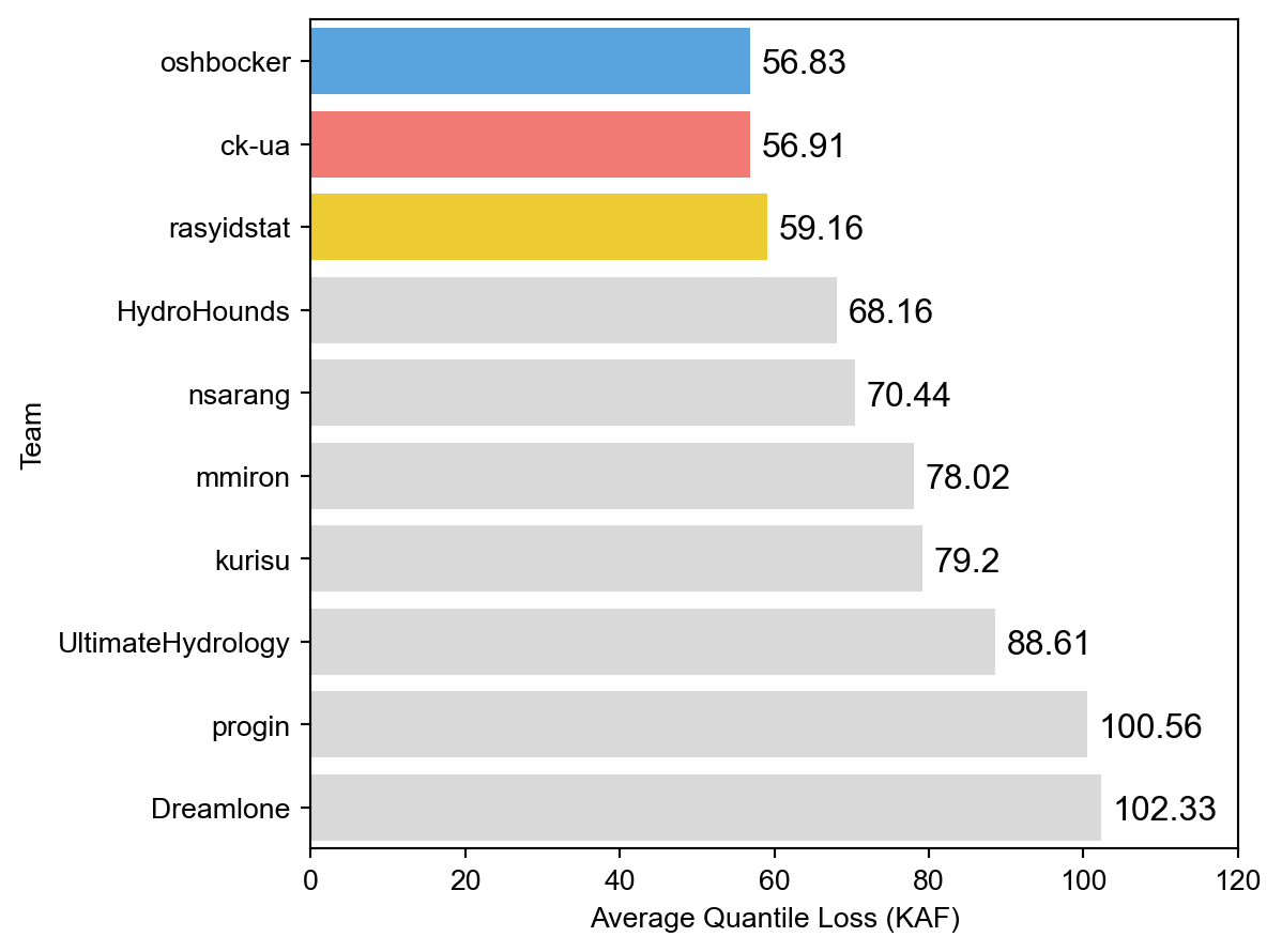
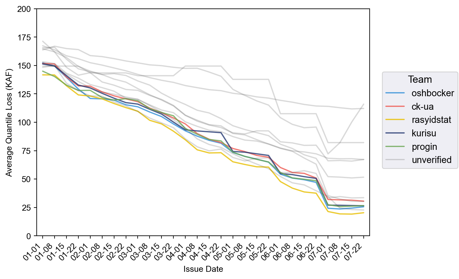
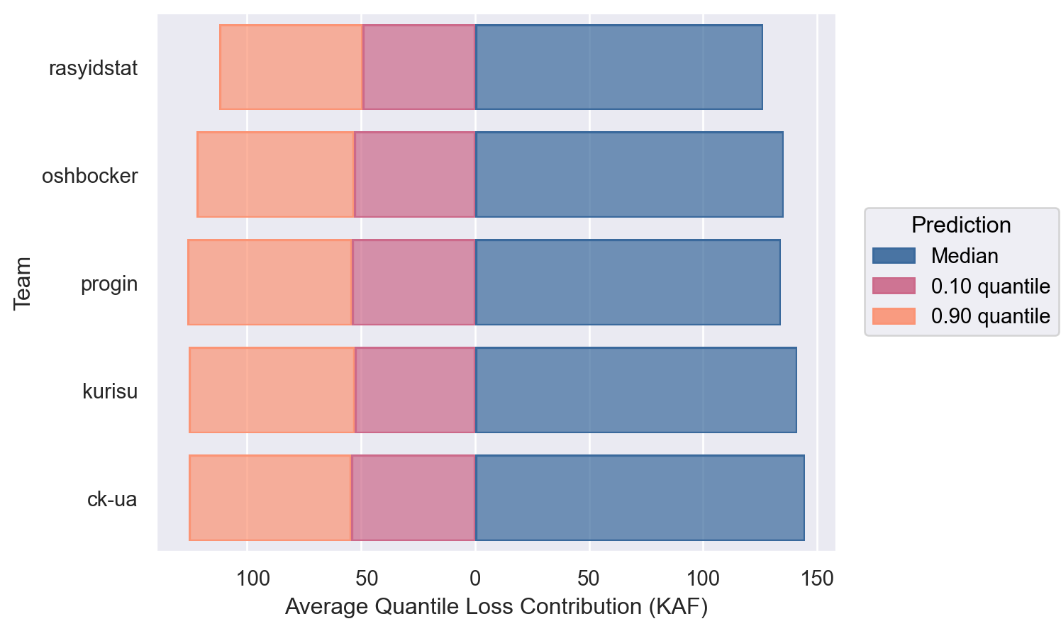
Most winners and other competitive solutions had cross-validation scores clustered in the range from 85–90 KAF, with 3rd place winner rasyidstat standing out with score of 79.5 KAF. This pattern in the averaged scores also holds throughout the year when breaking out the scores by issue date, shown below.
Among the winners, the highest skilled solutions by rasyidstat and oshbocker had both more accurate median point estimates and uncertainty bounds than the others. For progin, kurisu, and ck-ua, their solutions' uncertainty bounds were of relatively similar skill and primarily differentiated by their median point estimate performance. Unsurprisingly, the 0.10 quantile was easier to predict than the 0.90 since water supply volume is physically bounded from below at 0.
Here are a few takeaways from the winning solutions:
Tree-based models, particularly gradient-boosted trees, were highly represented among all submissions and particularly among winning teams, with a notable exception. All winners except the 2nd place team ck-ua used gradient-boosted trees, with frameworks including included LightGBM, XGBoost, and CatBoost. Team ck-ua stood out with their multilayer perceptron neural network model. This meant that all of the solutions with gradient-boosted trees approached the quantile regression with models independently predicting the three quantiles, while ck-ua's multilayer perceptron was able to produce predict all three at once.
Solutions favored pooling data across sites and across issue dates. Solvers also had a modeling choice on whether to develop separate models per site and separate models per issue date. These decisions trade off having models focused on a simpler task versus pooling more data together. Overall, we found that solvers tended to prefer pooling data both across all sites and across all issue dates. Among the winners, all had models for all sites, and all had models for all issue dates with the exception of 5th place progin, who trained models for each issue month.
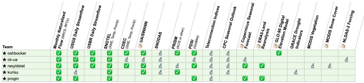
Winners converged on high-value predictor data sources. The challenge included a wide range of approved feature data, and solvers had the opportunity to experiment with many of them. The table below summarizes the data sources used and experimented with by the winners. Antecedent streamflow, snowpack measurements, and meteorological observations like precipitation and temperature were unsurprisingly key data sources for the winning models. Interestingly, many solvers experimented with the various approved climate teleconnection indicates, but none ended up in any of the winners' final models. There were also several cases where the challenge had approved two similar kinds of data products and one saw notably more success in models than the other. UA/SWANN and SNODAS—both spatially modeled snow water equivalent data products—were widely experimented with by solvers, with UA/SWANN ending up in three of the winning models and SNODAS not used in any. For drought indicators, the Palmer Drought Severity Index derived from GridMET data was used in three of the winning models, while GRACE-based indicators were not used in any. Seasonal forecasts from Copernicus (issued by ECMWF) were used in two winning models, while NOAA's Climate Prediction Center (CPC) were experimented with by four winners but not ultimately used. Finally, the ERA5-Land climate reanalysis dataset was used in two of the winning models, while the NCEP/NCAR reanalysis dataset was not used in any.
Results of the Explainability and Communication Bonus Track
In the Final Prize Stage, solvers could also compete for Explainability and Communication Bonus prizes by submitting example forecast summaries for water manager decision-makers. These forecast summaries were short documents—representative of real publications from forecasting agencies—that would provide context for and explanations of forecasted cumulative streamflow volume. Winners were evaluated by qualitative criteria by a panel of technical experts who evaluated solutions' usefulness, clarity, rigor, and innovation.
| Place | Team | Prize |
|---|---|---|
| 1st | kurisu | $25,000 |
| 2nd | kamarain | $20,000 |
| 3rd | rasyidstat | $15,000 |
| 4th | oshbocker | $10,000 |
| 5th | iamo-team | $5,000 |
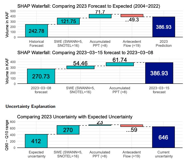
Successful forecast summaries had clear visualizations of forecast trends and contextual trends in key predictor variables over the year, with comparisons against historical baselines. SHAP values were a popular choice for feature importance among the winning solutions, with the top solutions particularly innovative uses of them. For 1st place winner kurisu, judges particularly liked the SHAP waterfall plots, shown below, which were used to explain not just deviation from the historical average but also changes from the previous forecast and the size of the uncertainty bounds. Judges also liked a SHAP visualization used by 2nd place winner kamarain which compared SHAP feature importance values for that forecast against historical average SHAP values.
Winning Solutions Code and Reports
All winning solution code and reports can be found in our winners repository on GitHub. All solutions are licensed under the open-source MIT license.
Meet the Winners
Matthew Aeschbacher

Total Prize: $155,000
Prizes Won: Final Prize Stage 1st Place Overall ($100,000), Challenging Basins Bonus ($10,000), and Explainability and Communication Bonus Track 4th Place ($10,000); Forecast Stage 1st Place ($25,000); Hindcast Stage 3rd Place ($10,000)
Hometown: Denver, Colorado
Username: oshbocker
Social Media: /in/matthewpaeschbacher/
Background:
I work as a Senior Machine Learning Engineer for Uplight, Inc. where I build production machine learning systems that help orchestrate energy assets on the electric grid.
What motivated you to compete in this challenge?
Growing up and living in Denver, Colorado I have long been aware of the importance of seasonal streamflow to communities across the Western United States. I wanted to take this opportunity to learn more about the dynamics that shape streamflow from season to season and help give back to the community.
Summary of modeling approach:
There are two model architectures underlying the solution, each one implemented using two different gradient boosting on decision trees methods (Catboost and LightGBM) for a total of four models. The first model architecture predicts the quantiles of total cumulative streamflow volume in each season, for each site. The second model architecture predicts the quantiles of monthly cumulative streamflow volume within the season, for each site. The monthly predicted quantiles are then summed over the season to give the seasonal streamflow volume. The models use static features from each site including, the latitude, longitude, elevation, and categorical site id. The models also use dynamic features including, the day of the year, and features derived from localized precipitation, temperature, streamflow measurement from streamgages, and snow water equivalent measurements. The quantile predictions from each model are combined using a regularized regression to minimize the prediction error given by the mean quantile loss across the three quantiles.
Summary of explainability approach:
The explainability reports provide contextual data and visualizations to help users understand what data is most influential for each stream site and how the model weighs that data in obtaining predictions. With an ensemble of up to 12 different models, we included visualizations offering insights from individual components and showing how the ensemble contributions combine. We used Shapley values for gradient boosted models and customized these explanations for our ensemble of quantile regressors. Our goal was to help users understand both how and why the model produced specific quantile predictions on a given date and reason about how changing conditions might impact future predictions.
Check out Matthew's full write-up and solution for the Forecast Stage challenge winners repository. The full write-up and solution for the Final Prize Stage are also in the repository, as is Matthew's forecast summaries, report, and code for the Explainability Bonus Track.
Rasyid Ridha

Total Prize: $140,000
Prizes Won: Final Prize Stage 3rd Place Overall ($50,000), Cascades Bonus ($10,000), Sierra Nevada Bonus ($10,000), Colorado Headwaters Bonus ($10,000), Early Lead Time Bonus ($10,000), and Explainability and Communication Bonus Track 3rd Place ($15,000); Forecast Stage 3rd Place ($10,000); Hindcast Stage 1st Place ($25,000)
Home country: Indonesia
Username: rasyidstat
Background:
Experienced Data Scientist specializing in time series and forecasting. Currently working in the IoT domain, focusing on elevating consumer experience and optimizing product reliability through data-driven insights and analytics. Previously worked in various tech companies in Indonesia.
What motivated you to compete in this challenge?
I was motivated to compete in this challenge because of its unique setup. Unlike typical data science competitions, there's no predefined training dataset provided. This means participants must not only focus on modeling but also on finding the right data to be used. Additionally, the requirement to submit operational code adds another layer of complexity and practical application. I saw this as an exciting opportunity to test and expand my machine learning skills in a practical, real-world setting.
Summary of approach:
We use an ensemble of LightGBM models with Tweedie loss for point forecast and quantile loss for 0.10 and 0.90 quantile forecast. We mainly use lagged data of SNOTEL/CDEC SWE and cumulative precipitation averaged within and near the basins from top 𝐾 = 9 SNOTEL/CDEC sites as the input of the model. In addition, for different ensemble members, we incorporate various gridded data products averaged within the basins, including gridMET PDSI, UA/SWANN SWE, ERA5-Land, and seasonal forecast products from ECMWF SEAS51. To mitigate small sample size problems, We use synthetic data generation and increase the training sample size by 5x, which significantly improves forecast skill, prediction interval reliability, and generalizability. We also incorporate daily USGS and USBR observed flow from sites with minimal impairment. Compared to the model in the Hindcast Stage, forecast skill has improved by ~5 KAF and it is attributed to additional data sources used and better estimates of snowpack in some regions, especially in Sierra Nevada and Cascades region.
Summary of explainability approach:
SHAP (SHapley Additive exPlanations) to calculate the percentage of feature contribution and relative contribution as explainability metrics for a given location and issue date. Forecast predictions are displayed with the initial forecast update in January, along with historical median, average, minimum, and maximum values. Explainability metrics are displayed with the latest two consecutive issue dates as a comparison, including values for each feature, typically expressed as percent of normal.
Check out Rasyid's full write-up and solution for the Forecast Stage challenge winners repository. The full write-up and solution for the Final Prize Stage are also in the repository, as is Rasyid's forecast summaries, report, and code for the Explainability Bonus Track.
Roman Chernenko and Vitaly Bondar


Total Prize: $105,000
Prizes Won: Final Prize Stage 2nd Place Overall ($75,000); Forecast Stage 2nd Place ($15,000); Hindcast Stage 2nd Place ($15,000)
Hometown: Cherkasy, Ukraine
Team name: ck-ua
Usernames: RomanChernenko, johngull
Social Media: /in/roman-chernenko-b272a361/, /in/vitalybondar/
Background:
Roman Chernenko: Machine Learning Engineer in Agreena ApS company with 4 years of experience in ML for geospatial applications, satellite imaging and precision agriculture. Also, I have 10 years of experience with C++ cross-platform development, especially in the medical imaging domain, and for embedded solutions.
Vitaly Bondar: ML Team lead in theMind (formerly Neuromation) company with 6 years of experience in ML/AI and almost 20 years of experience in the industry. Specialises in the CV and generative AI.
What motivated you to compete in this challenge?
The main motivation is a complicated, interesting challenge with a significant prize amount. Also, we participated in a similar challenge "Snowcast Showdown" at DrivenData 2 years ago and finished 6th.
Summary of approach:
Our approach centered on using a Multi-Layer Perceptron (MLP) neural network with four layers, which proved to be the most effective within the given constraints. The network was constructed to simultaneously predict the 10th, 50th, and 90th percentile targets of water level distribution. We experimented with various network enhancements and dropout regularization but observed no substantial improvement in the model's performance. For our data sources, we relied on the NRCS and RFCs monthly naturalized flow, USGS streamflow, USBR reservoir inflow and NRCS SNOTEL data, all of which were meticulously normalized and encoded to serve as features for our training process. We propose a novel approach for using SNOTEL data by training specialized RANSAC mini-models for each site separately. For each of these mini-models the list of the used SNOTEL stations are selected by heuristic approach. We also employed data augmentation due to the limited size of our training dataset, which allowed us to artificially expand our sample set.
Check out Team ck-ua's full write-up and solution for the Forecast Stage challenge winners repository. The full write-up and solution for the Final Prize Stage are also in the repository.
Christoph Molnar

Total Prize: $55,000
Prizes Won: Final Prize Stage Overall 4th Place ($30,000), Explainability and Communication Bonus Track 1st Place ($25,000),
Hometown: Munich, Germany
Username: kurisu
Website: christophmolnar.com
Background:
I write and self-publish books on machine learning with a focus on topics that go beyond just training the models, such as uncertainty quantification and interpretability. I have a background in statistics and machine learning.
What motivated you to compete in this challenge?
I love to write, but sometimes I need practical projects. Especially when writing practical books, I don't want to lose touch with the practical side of machine learning. The Water Supply Forecasting Rodeo fit that perfectly and checked many other boxes too: I am interested in all things earth system science, and the challenge had an additional bonus track on explainability and communication, as well as attractive prizes.
Summary of modeling approach:
Our water supply forecasting solution is based on quantile regression using gradient-boosted trees (xgboost). The models are trained for all sites and issue dates simultaneously. To predict each quantile, an ensemble of 10 xgboost models is used in combination with adjusting lower and upper quantiles to ensure an 80% interval coverage. Besides issue date and site, the models rely only on features describing snow conditions (SWANN, SNOTEL) and antecedent flow (NRCS, RFCs). Training takes 6 seconds, prediction is even faster, and the feature list is short and interpretable.
Summary of explainability approach:
When interpreting machine learning models, we used model-agnostic approaches that can be applied to any model. We employed Shapley values and What-if plots for both the forecasts and the uncertainty (measured as the range between 10% and 90% quantile). For explaining uncertainty, we redefined the interval range as the "prediction function". The communication outputs include Forecast Plots for visualizing water supply forecasts at different quantiles, along with Context Plots showing watershed conditions throughout the year compared to historical conditions (2004-2022).
Check out Christoph's full write-up and solution for the Final Prize Stage in the challenge winners repository. Also check out Christoph's forecast summaries, report, and code for the Explainability Bonus Track in the repository.
Piotr Rogiński

Total Prize: $20,000
Prizes Won: Final Prize Stage Overall 5th Place ($20,000)
Hometown: Gdańsk, Poland
Username: progin
Social Media: /in/piotr-roginski/
Background:
I am a data scientist with 3 years of commercial experience in sales, pharmacovigilance and insurance industries. I specialize in data processing, feature engineering and gradient boosting algorithms. I am currently looking for a job where I could work on machine learning problems more frequently.
What motivated you to compete in this challenge?
I wanted to participate in a data science competition where I could use my analytical and machine learning skills. Participating in a competition that tries to tackle real world problems was another motivation.
Summary of modeling approach:
I used LightGBM models as main predictors for each quantile and historical data distribution estimates for 0.1 and 0.9 quantile corrections. Best distribution was chosen for each reservoir to find optimal data representation and quantile values. A LightGBM prediction of quantile 0.5 was used as a center for the fitted distribution, from which other quantiles were calculated. The models were created separately for each month to enable better features as more information becomes available. For the last three months (May-July), I used known naturalized flow from past months and made forecasts to predict the remaining amount until July. I kept feature selection minimal, using no more than ten features per month due to the small training dataset. The solution includes clipping methods to keep forecasts within historical ranges and adjusts for cases where quantile ordering is violated or where known flow is similar to the total forecast.
Check out Piotr's full write-up and solution for the Final Prize Stage in the challenge winners repository.
Matti Kämäräinen
Total Prize: $20,000
Prizes Won: Explainability and Communication Bonus Track 2nd Place ($20,000)
Hometown: Helsinki, Finland
Username: kamarain
Background:
I work as a researcher and developer at the Finnish Meteorological Institute, mostly working on developing weather impact forecasting tools using machine learning.
What motivated you to compete in this challenge?
I have participated in these kinds of challenges previously with good success, most importantly the Streamflow Forecasting Rodeo a couple years ago. In that competition I was using the name salmiaki. I really like using the scientific approach to find a well performing model, even though it is quite a laborious task. The background knowledge of meteorology and related fields is an advantage.
Summary of explainability approach:
Our approach focused on creating one information-rich figure sufficient for presenting the previous and current model results for each target site and issue date, including historical observed quantiles of the naturalized flow for context. We followed a bottom-up strategy for explaining the competition forecasts. First, individual model features – the spatio-temporal principal components of each dataset – are explored with SHAP analysis to find out which ones contribute most to the predictions of each issue date and target site. Then the identified features are visualized and narrated together with the other features and datasets.
Check out Matti's forecast summaries, reports, and code in the challenge winners repository.
Atabek Umirbekov and Changxing Dong


Total Prize: $5,000
Prizes Won: Explainability and Communication Bonus Track 5th Place ($5,000)
Hometown: Halle, Germany
Team name: iamo-team
Background:
Atabek Umirbekov: Doctoral researcher at the Leibniz Institute of Agricultural Development in Transition Economies (IAMO). My research primarily deals with the impacts of climate variability and change on water resources and agricultural production in Central Asia.
Dr. Changxing Dong: Researcher in the Department Structural Change of IAMO. My research interests are Agent-Base modelling and application of Machine Learning in the domain of structural development of agricultural regions.
What motivated you to compete in this challenge?
Atabek's recent research focuses on improving seasonal water supply forecasting in Central Asia, a region geographically distant from the western US but sharing similar climate and hydrological dynamics: accumulated snowpack is the primary determinant of seasonal river flow.
Summary of explainability approach:
For each issue date, our forecast summaries present predictions of seasonal streamflow volumes putting them in historical context, alongside current conditions for key hydrological variables like basin snowpack, accumulated precipitation, and antecedent river flow. These summaries offer insights into the evolving prediction power of the used variables over the target water year, which is important for understanding forecasted streamflow volumes. We also address variations in the predictive power of these variables along all issue dates, accounting for factors like basin characteristics and issue date timing by including information on their relevance derived from the forecast model using a model-agnostic method.
Check out iamo-team's forecast summaries, reports, and code in the challenge winners repository.
Thanks to all the participants and to our winners! Thanks also to Bureau of Reclamation for sponsoring this challenge, and our other collaborators from the Natural Resources Conservation Service, the U.S. Army Corps of Engineers, and the NASA Tournament Lab. Special thanks to the judging panels: Angus Goodbody (NRCS), Christopher Frans (USBR), Kevin Foley (NRCS), Navead Jensen (USBR), Michael Warner (USACE), Paul Miller (NOAA CBRFC), Austin Balser (USBR), Claudia Leon Salazar (USBR), Clayton Jordan (USBR), George Finnegan (USBR), and Tara Campbell Miranda (USBR).
Thumbnail and banner image is a photograph of Hungry Horse Dam in Montana. Image courtesy of USBR.