Welcome! This guest post from our partners at the MIT Gabrieli Lab will guide you through building a simple baseline model for the Goodnight Moon, Hello Early Literacy Screening Challenge. This benchmark will predict scores for literacy screening tasks using extracted audio features. For access to the data used in this benchmark notebook, sign up for the competition here.
This notebook will:
- Load the dataset
- Perform exploratory data analysis
- Create feature representations
- Split the data into train and test sets
- Train an XGBoost model
- Predict and evaluate locally
- Prepare model code and assets for submission
Background
Literacy skills are critical to a child’s success in school and beyond, yet a significant portion of students in the US are struggling with reading abilities. Early intervention is crucial, but the current approach to literacy screening in classrooms relies heavily on teachers administering and manually scoring assessments—a process that can be time-consuming and sometimes inconsistent due to variations in scorer training and interpretation.
Reach Every Reader has developed a comprehensive literacy screening assessment. This assessment includes tasks designed to measure key language skills, such as phonological awareness and working memory. Specifically, tasks like deletion, blending, nonword repetition, and sentence repetition capture critical aspects of early literacy development. While the information gathered from these tasks is invaluable, the manual scoring process limits its potential impact.
This competition invites participants to develop machine learning models that can automatically and accurately score these audio-based literacy tasks. By building reliable models, competitors can help ease administrative load on teachers, increase scoring accuracy, and ensure more consistent support for students at risk.
Let's get started!
# Built-ins
import joblib
from pathlib import Path

# Audio processing libraries
import librosa
import librosa.display
import opensmile
import webrtcvad

# Machine learning and data handling
import numpy as np
import pandas as pd
from sklearn.model_selection import train_test_split
from sklearn.calibration import CalibratedClassifierCV
from sklearn.metrics import log_loss
from tqdm import tqdm
import xgboost as xgb
from xgboost import XGBClassifier

# Visualization
import matplotlib.pyplot as plt
Step 1: Load the Data
Ensure that the train_labels.csv file is available in the data/ folder before running this step. In this setup, the audio files are in a subfolder in data/ called audio/. You can change the paths to match your setup.
DATA_PATH = Path("data")
AUDIO_PATH = DATA_PATH / "audio"
labels = pd.read_csv(DATA_PATH / "train_labels.csv")
print(f"Train labels shape: {labels.shape}")
labels.head()
metadata = pd.read_csv(DATA_PATH / "train_metadata.csv")
print(f"Train metadata shape: {metadata.shape}")
metadata.head()
We'll join these datasets together to help with our exploratory data analysis.
df = labels.merge(metadata, on="filename", validate="1:1")
print(f"df shape: {df.shape}")
df.head()
Step 2: Exploratory Data Analysis
We will now explore the dataset and visualize some features.
def plot_waveform(filepath):
    # Load the audio file
    audio_data, sr = librosa.load(filepath, sr=None)

    # Plot the waveform
    plt.figure(figsize=(10, 4))
    librosa.display.waveshow(audio_data, sr=sr)
    plt.title("Waveform")
    plt.xlabel("Time (s)")
    plt.ylabel("Amplitude")
    plt.show()

    return audio_data, sr
def plot_spectrogram(audio_data, sr):
    # Generate the spectrogram
    S = librosa.stft(audio_data)
    S_db = librosa.amplitude_to_db(np.abs(S), ref=np.max)

    # Plot the spectrogram
    plt.figure(figsize=(10, 4))
    librosa.display.specshow(S_db, sr=sr, x_axis="time", y_axis="log")
    plt.colorbar(format="%+2.0f dB")
    plt.title("Spectrogram")
    plt.xlabel("Time (s)")
    plt.ylabel("Frequency (Hz)")
    plt.show()
def voice_activity_detection(filepath, aggressiveness=2):
    vad = webrtcvad.Vad(aggressiveness)  # Aggressiveness from 0 to 3
    audio_data, sr = librosa.load(filepath, sr=16000)  # VAD prefers 16kHz audio
    audio_data = (audio_data * 32767).astype(np.int16)  # Scale to int16 for VAD

    frame_duration = 30  # Frame duration in ms
    frame_length = int(sr * frame_duration / 1000)

    # Collect VAD results
    vad_results = []
    for start in range(0, len(audio_data), frame_length):
        frame = audio_data[start : start + frame_length].tobytes()
        vad_results.append(vad.is_speech(frame, sr))

    # Plot VAD output
    time_axis = np.linspace(0, len(audio_data) / sr, num=len(vad_results))
    plt.figure(figsize=(10, 2))
    plt.plot(time_axis, vad_results, label="VAD Output")
    plt.title("Voice Activity Detection (VAD) Output")
    plt.xlabel("Time (s)")
    plt.ylabel("Speech Detected")
    plt.ylim(-0.1, 1.1)
    plt.show()
def analyze_audio(filepath):
    print("Plotting waveform...")
    audio_data, sr = plot_waveform(filepath)

    print("Plotting spectrogram...")
    plot_spectrogram(audio_data, sr)

    print("Performing Voice Activity Detection...")
    voice_activity_detection(filepath)
Let’s take a closer look at each task and its selected examples. For each task, we analyze paired examples — one correct and one incorrect — to better understand how variations in responses manifest in the dataset.
Deletion
Deletion evaluates a child’s phonological awareness by asking them to listen to a word and then delete part of it to form a new, sensical word. In this example, the child is prompted with “haircut without cut,” and the expected response is “hair.” In the audio file gpksml.wav, the child provides an incorrect response by providing the response "cut", failing to accurately produce the target word “hair.”
incorrect_deletion = "gpksml.wav"

df[df.filename == incorrect_deletion]
analyze_audio(AUDIO_PATH / incorrect_deletion)
In contrast, the audio file faudzc.wav demonstrates a correct response to the same task. The child successfully identifies and removes the portion “cut” from “haircut” to produce “hair,” indicating strong phonological awareness and the ability to modify spoken words accurately.
correct_deletion = "faudzc.wav"

df[df.filename == correct_deletion]
analyze_audio(DATA_PATH / "audio" / correct_deletion)
Sentence Repetition
Sentence repetition assesses the child’s ability to replicate a sentence verbatim, maintaining both structure and meaning. In this case, the sentence is “ring the bell on the desk to get her attention.” The response in khlzie.wav modifies the wording slightly, saying “ring the bell on her desk to get her attention,” which is marked incorrect due to the deviation from the original. While the meaning remains somewhat intact, the structural deviation marks it as incorrect.
incorrect_sentrep = "khlzie.wav"
df[df.filename == incorrect_sentrep]
analyze_audio(AUDIO_PATH / incorrect_sentrep)
The correct response in loqrbr.wav accurately replicates the entire sentence without any alterations, demonstrating the child’s strong linguistic processing and auditory memory skills.
correct_sentrep = "loqrbr.wav"
df[df.filename == correct_sentrep]
analyze_audio(AUDIO_PATH / correct_sentrep)
Nonword Repetition
Nonword repetition evaluates phonological working memory by asking the child to repeat a nonsensical word. In this case, the child was asked to repeat “gowfdoikeem.” The response in dxpwed.wav contains slight phonetic inaccuracies, leading to an incorrect score.
incorrect_nonword = "dxpwed.wav"
df[df.filename == incorrect_nonword]
analyze_audio(AUDIO_PATH / incorrect_nonword)
In contrast, the response in bnafxc.wav correctly reproduces the nonword “gowfdoikeem,” showcasing the child’s ability to retain and articulate unfamiliar sound patterns. This indicates strong phonological working memory.
correct_nonword = "bnafxc.wav"
df[df.filename == correct_nonword]
analyze_audio(AUDIO_PATH / correct_nonword)
Blending
Blending assesses the child’s ability to combine separate phonemes to form a complete word. In this example, the task asks the child to blend the sounds m - ou - se to produce “mouse.” The response in hvqvny.wav includes slight phonetic differences, which result in an incorrect response.
incorrect_blending = "hvqvny.wav"
df[df.filename == incorrect_blending]
analyze_audio(AUDIO_PATH / incorrect_blending)
The correct response in jkvyty.wav illustrates a successful blending of the same sounds m - ou - se into the target word “mouse.” This response shows phonological awareness and ability to process sounds accurately.
correct_blending = "jkvyty.wav"
df[df.filename == correct_blending]
analyze_audio(AUDIO_PATH / correct_blending)
Step 3: Feature Engineering
In this step, we will generate features that will be used by our model.
The eGeMAPS (Extended Geneva Minimalistic Acoustic Parameter Set) feature set is a tool for analyzing speech and is implemented through the openSMILE framework (open-source Speech and Music Interpretation by a Large collection of Extractors). This toolkit extracts 88 key acoustic features, focusing on elements like pitch, loudness, and pauses, which are critical for evaluating speech clarity and fluency.
eGeMAPS is compact but highly effective, capturing important speech features while remaining efficient. Its wide use in speech research makes it a strong fit for scoring literacy assessments. By leveraging openSMILE, we provide our model with detailed, meaningful data.
# Initialize OpenSMILE with eGeMAPS configuration for extracting features
smile = opensmile.Smile(
    feature_set=opensmile.FeatureSet.eGeMAPSv02,  # Use eGeMAPS for feature extraction
    feature_level=opensmile.FeatureLevel.Functionals,  # Extract summary statistics
)
# Extract features with tqdm progress bar
feature_list = []
for filename in tqdm(df.filename, desc="Extracting OpenSMILE Features", unit="file"):
    features = smile.process_file(AUDIO_PATH / filename)  # Extract features for each file
    feature_list.append(features.mean(axis=0))  # Take the mean across time for stability
# Convert extracted features to DataFrame
X = pd.DataFrame(feature_list, index=df.filename)

# Set up target variable
y = df.score
Step 4: Train-Test Split
We will split the data into training and testing sets to evaluate the model.
X_train, X_test, y_train, y_test = train_test_split(X, y, test_size=0.2, random_state=42)

print(f"Training set size: {X_train.shape}")
print(f"Test set size: {X_test.shape}")
Step 5: Train a Baseline Model
We will train a simple XGBoost classifier using the generated features and evaluate its performance.
# Initialize and train the XGBoost model
xgb_model = XGBClassifier(n_estimators=100, random_state=42, eval_metric="logloss")

calibrated_model = CalibratedClassifierCV(xgb_model, cv=3)
calibrated_model.fit(X_train, y_train)

# Make predictions and evaluate using log loss
y_pred_proba = calibrated_model.predict_proba(X_test)[
    :, 1
]  # Probability of 'correct' (class 1)
logloss = log_loss(y_test, y_pred_proba)
print(f"Log Loss on the test set: {logloss}")
Since this is a code execution competition, we will submit our model weights and code rather than predictions. Let's first train our model on the full training set (X) instead of the 80% split (X_train) we used for local iteration.
calibrated_model.fit(X, y)
Step 6: Write main.py and save out assets for submission
Now that we have a trained model, we will package up our model and inference code for predicting on the test set in the runtime container. Predictions will be written out in the expected submission.csv format. For more details, see the Code Submission Format page.
Submission format requirements
- Your submission must be a
.ziparchive (e.g.,submission.zip) containing amain.pyfile at the root level. - The
main.pyscript should:- Load your pretrained model (which should be included in your submission) and perform inference on the test audio clips.
- Write predictions to a file named
submission.csvin the same directory asmain.py.
Competition runtime limits
Before preparing your submission, please ensure you understand the runtime environment and its constraints:
- Your submission must run using Python 3.12 with packages specified in the runtime repository.
- The submission must complete execution within 4 hours or less. Most submissions are expected to run much faster.
- The runtime container provides access to a single GPU. All code must execute within the GPU environment, although computations may still occur on the CPU. (A CPU environment is available within the container for local debugging.)
- The container has access to the following resources:
- 16 vCPUs
- 110GB RAM
- A single NVIDIA T4 GPU with 16GB VRAM
- The container does not have network access. All required files, including code and model assets, must be included in your submission.
- The container execution will not have root access to the filesystem.
Please ensure your submission complies with these limits to guarantee successful execution.
Preparing our submission
Our first step will be to save out the calibrated XGBoost model we have just trained on the entire training dataset. We will save this out as a .joblib file, though there are other formats you can use.
ASSETS_DIR = Path("assets")
ASSETS_DIR.mkdir(exist_ok=True)

joblib.dump(calibrated_model, ASSETS_DIR / "calibrated_model.joblib")
Now we'll write out our main.py file. Below is an example of a properly formatted main.py file that runs our model pipeline:
import joblib
from pathlib import Path

import opensmile
import pandas as pd


DATA_PATH = Path("data")


def main():
    # load submission format
    sub_format = pd.read_csv("data/submission_format.csv", index_col="filename")

    # initialize OpenSMILE with eGeMAPS configuration for extracting features
    smile = opensmile.Smile(
        feature_set=opensmile.FeatureSet.eGeMAPSv02,  # Use eGeMAPS for feature extraction
        feature_level=opensmile.FeatureLevel.Functionals  # Extract summary statistics
    )

    # create features
    feature_list = []
    for filename in sub_format.index:
        features = smile.process_file(DATA_PATH / filename)  # extract features for each file
        feature_list.append(features.mean(axis=0))  # take the mean across time for stability

    features = pd.DataFrame(feature_list, index=sub_format.index)

    # load model
    model = joblib.load("assets/calibrated_model.joblib")

    # make predictions
    preds =  model.predict_proba(features)[:, 1]

    # write out to submission format
    sub_format["score"] = preds
    sub_format.to_csv("submission.csv")


if __name__ == "__main__":
    main()
Step 7: Test your submission locally
The competition provides a streamlined process for testing submissions locally using a Docker container that mimics the runtime environment. To ensure your submission works correctly, you can test it locally using the competition's runtime repository. Since there are detailed instructions in the README, we'll just provide a concise guide here.
Clone the runtime repo:
git clone https://github.com/drivendataorg/literacy-screening-runtime.git
Download the official competition Docker image:
make pullSet up your data directory:
- Download the smoke test data from the data download page
- Extract this into your
data/directory for local testing with:tar xzvf smoke.tar.gz --strip-components=1 -C data/
- In the local container,
/code_execution/datais a mounted version of your localdata/folder. The official runtime replaces this with the actual test data.
Prepare your submission:
- Save all submission files (e.g.,
main.py, model weights) in thesubmission_srcfolder. - Create the
submission.zipfile with:make pack-submission
- Save all submission files (e.g.,
Run your submission locally against the smoke test data:
- Test your submission in the runtime container:
make test-submission - This runs your
main.pyscript in the container and generatessubmission.csvin thesubmission/folder. - Use the logs saved in
submission/log.txtto debug any errors. These logs will help you identify issues with your code or the runtime environment.
- Test your submission in the runtime container:
Make sure your code runs smoothly locally before submitting to the competition platform!
Step 8: Submit to the competition!
Now that we've saved out our model and written our main.py, this is what our submission_src directory looks like:
❯ tree submission_src
submission_src
├── assets
│   └── calibrated_model.joblib
└── main.py
Let's generate our submission zipfile with make pack-submission:
❯ make pack-submission
mkdir -p submission/
cd submission_src; zip -r ../submission/submission.zip ./*
  adding: assets/ (stored 0%)
  adding: assets/calibrated_model.joblib (deflated 65%)
  adding: main.py (deflated 52%)
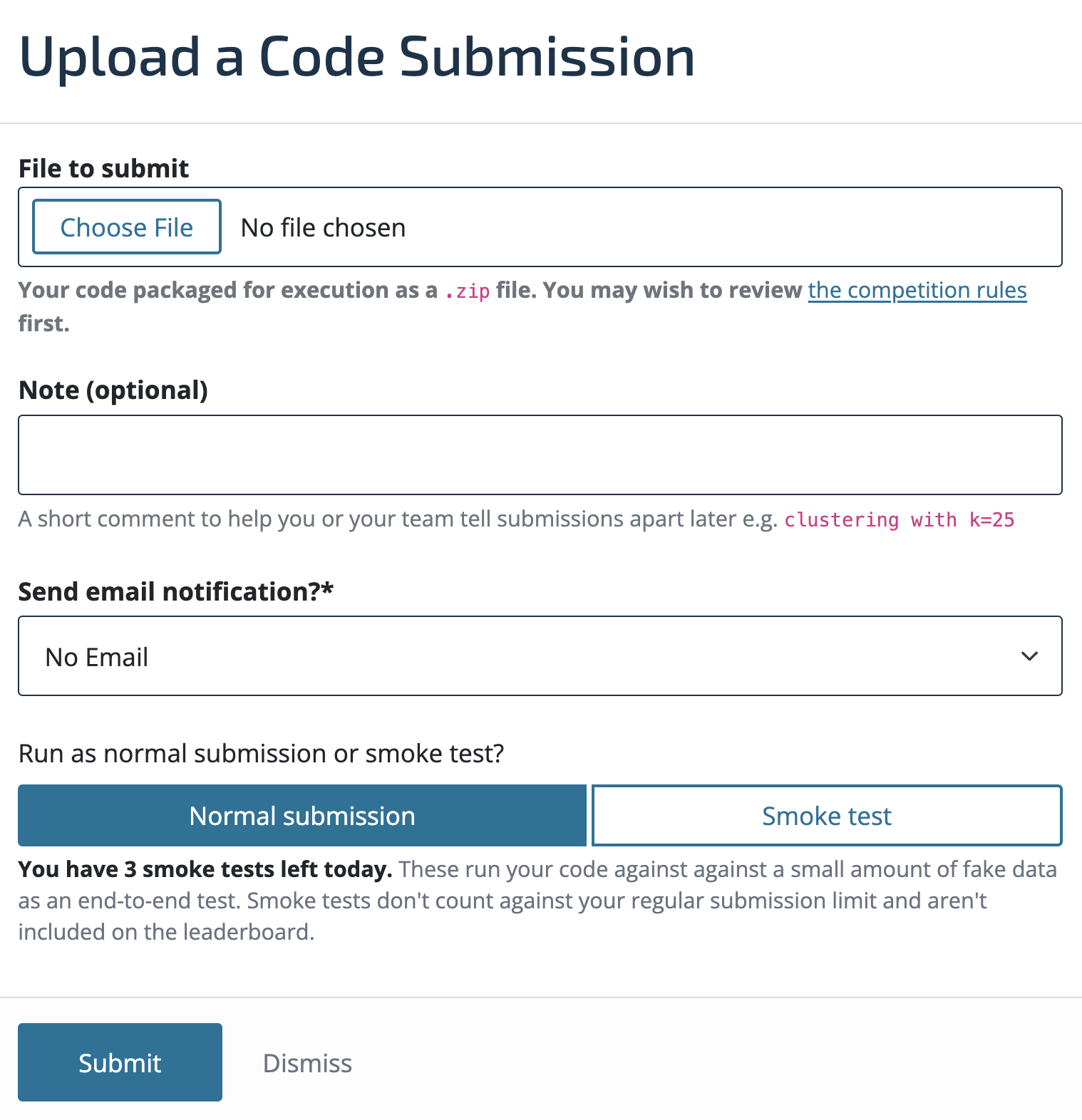
Now we're ready to submit our submission.zip to the competition! We've got the option of submitting a normal submission or smoke test. Smoke tests run your submission against a small subset of the training data for faster debugging. These tests won’t count for prizes but are helpful for identifying errors. You should run a smoke test submission before a normal submission to ensure your code executes properly.
Benchmark submission score
Our benchmark model achieved a log loss of 0.6063 and an AUROC of 0.7327. While there’s room for improvement, these results demonstrate the model’s potential for automating literacy task scoring and provide a strong foundation for further refinement.
Conclusion
This notebook provides a foundational pipeline for building a machine learning model for the Goodnight Moon, Hello Early Literacy Screening Challenge. It demonstrates how to preprocess the dataset, extract meaningful features, and train a benchmark model. While this is a strong starting point, there are many opportunities to improve performance by experimenting with advanced feature engineering, alternative model architectures, and optimized hyperparameters.
This challenge represents an exciting opportunity to make a tangible impact on early childhood education by helping automate and improve literacy assessments. We encourage you to iterate on this approach, explore innovative ideas, and push the boundaries of what machine learning can achieve in this domain.
If you want to share any of your findings or have questions, feel free to post on the community forum.
Good luck, and we’re excited to see how your models contribute to improving literacy outcomes!
