How to Use Deep Learning, PyTorch Lightning, and the Planetary Computer to Predict Cloud Cover in Satellite Imagery

Welcome to the benchmark notebook for the On Cloud N: Cloud Cover Detection Challenge! If you are just getting started, check out competition homepage. The goal of this benchmark is to:
- Demonstrate how to explore and work with the data
- Provide a basic framework for building a model
- Demonstrate how to package your work correctly for submission
You can either expand on and improve this benchmark, or start with something completely different! Let's get started.
Satellite imagery is critical for a wide variety of applications from disaster management and recovery, to agriculture, to military intelligence. Clouds present a major obstacle for all of these use cases, and usually have to be identified and removed from a dataset before satellite imagery can be used. Improving methods of identifying clouds can unlock the potential of an unlimited range of satellite imagery use cases, enabling faster, more efficient, and more accurate image-based research.
In this challenge, your goal is to detect cloud cover in satellite imagery.
The challenge uses publicly available satellite data from the Sentinel-2 mission, which captures wide-swath, high-resolution, multi-spectral imaging. For each tile, data is separated into 13 spectral bands capturing the full visible spectrum, near-infrared, and infrared light. Feature data is shared through Microsoft's Planetary Computer.
The ground truth labels for cloud cover are part of a new dataset created by Radiant Earth Foundation. After the competition ends, the labels dataset will be made publicly available to contribute to ongoing learning and advancement in the field.
In this post, we'll cover:
%load_ext autoreload
%autoreload 2
import shutil

import matplotlib.pyplot as plt
import numpy as np
import pandas as pd
from pandas_path import path
from pathlib import Path
from PIL import Image
import pytorch_lightning as pl
import torch
Explore the data
First, we'll download all of the competition data to a local folder. For instructions, see the competition's data download page. You'll need to join the competition in order to view the data page.
Data directory contents:
.
├── train_features
│   ├── train_chip_id_1
│   │   ├── B02.tif
│   │   ├── B03.tif
│   │   ├── B04.tif
│   │   └── B08.tif
│   └── ...
├── train_metadata.csv
└── train_labels
    ├── train_chip_id_1.tif
└── ...DATA_DIR = Path.cwd().parent.resolve() / "data/final/public"
TRAIN_FEATURES = DATA_DIR / "train_features"
TRAIN_LABELS = DATA_DIR / "train_labels"
assert TRAIN_FEATURES.exists()
The training data consists of 11,748 "chips". Each chip is imagery of a specific area captured at a specific point in time. There are four images associated with each chip in the competition data. Each image within a chip captures light from a different range of wavelengths, or "band". For example, the B02 band for each chip shows the strengh of visible blue light, which has a wavelength around 492 nanometers (nm). The bands provided are:
| Band | Description | Center wavelength |
|---|---|---|
| B02 | Blue visible light | 497 nm |
| B03 | Green visible light | 560 nm |
| B04 | Red visible light | 665 nm |
| B08 | Near infrared light | 835 nm |
Let's set a global variable with the list of bands in our training data, so it's easier to iterate over them for future steps.
BANDS = ["B02", "B03", "B04", "B08"]
Metadata
Let's start by looking at the metadata for the train set, to understand what the images in this competition capture.
train_meta = pd.read_csv(DATA_DIR / "train_metadata.csv")
train_meta.head()
# how many different chip ids, locations, and datetimes are there?
train_meta[["chip_id", "location", "datetime"]].nunique()
We have one row per chip, and each chip_id is unique. There are columns for:
location: General location of the chipdatetime: Date and time the satellite image was capturedcloudpath: All of the satellite images for this competition are hosted on Azure Blob Storage containers. You can use thiscloudpath, combined with the provideddownload_data.pyscript, to download any single chip from the container using the cloudpathlib library. You can also download all of the data at once, rather than chip by chip. See thedata_download_instructions.txtfile attached to the Data Download page for details.
Let's take a look at the distribution of chips by location.
train_location_counts = (
    train_meta.groupby("location")["chip_id"].nunique().sort_values(ascending=False)
)
plt.figure(figsize=(12, 4))
train_location_counts.head(25).plot(kind="bar", color="lightgray")
plt.xticks(rotation=90)
plt.xlabel("Location")
plt.ylabel("Number of Chips")
plt.title("Number of Train Chips by Location (Top 25)")
plt.show()
The train and test images are from all over the world! Location names can be countries (eg. Eswatini), cities (eg. Lusaka), or broader regions of a country (eg. Australia - Central). Sentinel-2 flies over the part of the Earth between 56° South and 82.8° North, between Cape Horn and slightly north of Greenland, so our observations are all between these two latitudes. The chips are mostly in Africa and South America, with some in Australia too.
We also have a timestamp for each chip. What is the time range in the data?
train_meta["datetime"] = pd.to_datetime(train_meta["datetime"])
train_meta["year"] = train_meta.datetime.dt.year
train_meta.groupby("year")[["chip_id"]].nunique().sort_index().rename(
    columns={"chip_id": "chip_count"}
)
train_meta["datetime"].min(), train_meta["datetime"].max()
chips_per_locationtime = (
    train_meta.groupby(["location", "datetime"])[["chip_id"]]
    .nunique()
    .sort_values(by="chip_id", ascending=False)
    .rename(columns={"chip_id": "chip_count"})
)
chips_per_locationtime.head(10)
All of the images in the data were captured between February of 2018 and September of 2020. We can also see from the training data that many chips share the same location and time.
We know from the problem description that all of the locations in the test set are new, and there is no overlap between locations in the train set and the test set.
Images
Next, let's explore the actual satellite images - the star of the show for this challenge!
For convenience, let's first add the paths to all of the feature images per chip. Remember, the folder for each chip has four images, each of which corresponds to a different band of light wavelengths.
def add_paths(df, feature_dir, label_dir=None, bands=BANDS):
    """
    Given dataframe with a column for chip_id, returns a dataframe with a column
    added indicating the path to each band's TIF image as "{band}_path", eg "B02_path".
    A column is also added to the dataframe with paths to the label TIF, if the
    path to the labels directory is provided.
    """
    for band in bands:
        df[f"{band}_path"] = feature_dir / df["chip_id"] / f"{band}.tif"
        assert df[f"{band}_path"].path.exists().all()
    if label_dir is not None:
        df["label_path"] = label_dir / (df["chip_id"] + ".tif")
        assert df["label_path"].path.exists().all()

    return df


train_meta = add_paths(train_meta, TRAIN_FEATURES, TRAIN_LABELS)
train_meta.head()
Each image is a GeoTIFF, a raster image file that contains geographic metadata. This metadata can include coordinates, an affine transform, and a coordinate reference system (CRS) projection. The package rasterio makes it easy to interact with our geospatial raster data.
Lets look at the red visible band (B04) image for a random chip.
import rasterio
example_chip = train_meta[train_meta["chip_id"] == "pbyl"]

display(example_chip)
The example chip is an image taken from Lodwar, a northwestern town in Kenya.
example_chip = example_chip.iloc[0]
with rasterio.open(example_chip["B04_path"]) as img:
    chip_metadata = img.meta
    img_array = img.read(1)

chip_metadata
We can see that the features are single-band images, with a shape of 512 x 512. The pixel values for each image measure the strength of light reflected back to the satellite for the specific set of wavelengths in that band. The array below shows the strength of red visible light, with wavelengts around 665 nm.
We can also see that there are no missing values in the image. This should be the case for all of the provided competition feature data.
# what does the image array look like?
print("Image array shape:", img_array.shape)
img_array
np.isnan(img_array).sum()
plt.imshow(img_array)
plt.title(f"B04 band for chip id {example_chip.chip_id}")
plt.show()
Coordinates
Using the metadata returned by rasterio, we can also get longitude and latitude coordinates.
# longitude/latitude of image's center
with rasterio.open(example_chip["B04_path"]) as img:
    lon, lat = img.lnglat()
    bounds = img.bounds
print(f"Longitude: {lon}, latitude: {lat}")
bounds
We have the longitude and latitude of the center of the image, but the bounding box values look very different. That's because the bounding box is given in whatever coordinate reference system the image is projected in, rather than traditional longitude and latiude. We can see which system with the crs value from the metadata.
We can convert the bounding box to longitude and latitude using pyproj.
import pyproj
def lat_long_bounds(filepath):
    """Given the path to a GeoTIFF, returns the image bounds in latitude and
    longitude coordinates.

    Returns points as a tuple of (left, bottom, right, top)
    """
    with rasterio.open(filepath) as im:
        bounds = im.bounds
        meta = im.meta
    # create a converter starting with the current projection
    current_crs = pyproj.CRS(meta["crs"])
    crs_transform = pyproj.Transformer.from_crs(current_crs, current_crs.geodetic_crs)

    # returns left, bottom, right, top
    return crs_transform.transform_bounds(*bounds)
left, bottom, right, top = lat_long_bounds(example_chip["B04_path"])
print(f"Image coordinates (lat, long):\nStart: ({left}, {bottom})\nEnd: ({right}, {top})")
True color image
We can make a composite image from the three visible bands (blue, green, and red) to visualize a high-quality, true color image. To show the true color image, we'll use the xarray and xrspatial packages designed for Sentinel-2 satellite data.
import xarray
import xrspatial.multispectral as ms
def get_xarray(filepath):
    """Put images in xarray.DataArray format"""
    im_arr = np.array(Image.open(filepath))
    return xarray.DataArray(im_arr, dims=["y", "x"])


def true_color_img(chip_id, data_dir=TRAIN_FEATURES):
    """Given the path to the directory of Sentinel-2 chip feature images,
    plots the true color image"""
    chip_dir = data_dir / chip_id
    red = get_xarray(chip_dir / "B04.tif")
    green = get_xarray(chip_dir / "B03.tif")
    blue = get_xarray(chip_dir / "B02.tif")

    return ms.true_color(r=red, g=green, b=blue)
fig, ax = plt.subplots(figsize=(5, 5))
im = true_color_img(example_chip.chip_id)
ax.imshow(im)
plt.title(f"True color image for chip id {example_chip.chip_id}")
That's a pretty high quality image!
Let's look at a few random training chips and their cloud labels.
def display_random_chip(random_state):
    fig, ax = plt.subplots(1, 2, figsize=(8, 4))
    random_chip = train_meta.sample(random_state=random_state).iloc[0]
    ax[0].imshow(true_color_img(random_chip.chip_id))
    ax[0].set_title(f"Chip {random_chip.chip_id}\n(Location: {random_chip.location})")
    label_im = Image.open(random_chip.label_path)
    ax[1].imshow(label_im)
    ax[1].set_title(f"Chip {random_chip.chip_id} label")

    plt.tight_layout()
    plt.show()
display_random_chip(1)
display_random_chip(9)
display_random_chip(40)
From the example chips, we can see that there is a very big variation in the amount of cloud cover per chip. The chip from Riobamba, Ecuador is almost completely obscured by clouds, while the chip from Macapá, Brazil has almost none.
Split the data
To train our model, we want to separate the data into a "training" set and a "validation" set. That way we'll have a portion of labelled data that was not used in model training, which can give us a more accurate sense of how our model will perform on the competition test data. Remember, none of the test set locations are in competition training data, so your model's will performance will ultimately be measured on unseen locations.
We have chosen the simplest route, and split our training chips randomly into 1/3 validation and 2/3 training. You may want to think about splitting by location instead of by chip, to better check how your model will do in new settings.
import random
random.seed(9)  # set a seed for reproducibility

# put 1/3 of chips into the validation set
chip_ids = train_meta.chip_id.unique().tolist()
val_chip_ids = random.sample(chip_ids, round(len(chip_ids) * 0.33))

val_mask = train_meta.chip_id.isin(val_chip_ids)
val = train_meta[val_mask].copy().reset_index(drop=True)
train = train_meta[~val_mask].copy().reset_index(drop=True)

val.shape, train.shape
# separate features from labels
feature_cols = ["chip_id"] + [f"{band}_path" for band in BANDS]

val_x = val[feature_cols].copy()
val_y = val[["chip_id", "label_path"]].copy()

train_x = train[feature_cols].copy()
train_y = train[["chip_id", "label_path"]].copy()
val_x.head()
val_y.head()
Code Execution Format
Rather than just generating predictions, this benchmark will show you how to create a correct submission for code execution. Your final submission will be a zipped archive called submission.zip. We'll create a folder called benchmark_src, and develop a complete code execution submission in that folder. benchmark_src will ultimately include:
The weights for our trained model
A
main.pyscript that loads the model, performs inference on images stored indata/test_features, generates chip-level predictions, and saves them out topredictions/. File names should match the chip IDs from the test dataset. For example, if the test set includes a chip with IDabcd, runningmain.pymust write out a predicted cloud cover TIF mask topredictions/abcd.tif. The predictions should be .tifs with values of1and0indicating cloud or no cloud.Any additional scripts that
main.pyneeds in order to run
main.py must be able to run without getting any input arguments, so make sure you set all your defaults so that calling python main.py alone runs the full process. Your final submission should not include prediction files.
All of the key code for inference is written out to scripts in benchmark_src using the line magic %%file instead of being run directly in this notebook. The final scripts that are written out by this notebook are also saved in a folder of the runtime repo.
# create benchmark_src folder
submission_dir = Path("benchmark_src")
if submission_dir.exists():
    shutil.rmtree(submission_dir)

submission_dir.mkdir(parents=True)
We'll run inference in this notebook by importing classes and functions from the scripts in benchmark_src.
Build the model
As a starting point, we'll build a basic neural network model using some of the standard libraries. That way there's lots of room for you to make improvements!
We'll use PyTorch Lightning, a package that introduces useful conventions for training deep learning models on top of PyTorch. Our model will start with a publicly available convolutional neural network called U-Net that is pretrained for semantic segmentation.
U-Net was first designed to help process biomedical imaging and identify things like signs of disease. The basic structure is an encoder network followed by a decoder network. We'll use a pretrained backbone called ResNet34 as our encoder.
CloudDataset
The first step of building the model is actually writing a class that will tell the model how to handle our feature data. Thankfully, the PyTorch Dataset and DataLoader classes take care of most of this for us! A Dataset object allows us to define custom methods for working with the data, and a DataLoader object parallelizes data loading. If you haven't worked with these classes before, we highly recommend this short tutorial.
We'll write a custom dataset called CloudDataset that reads our satellite image training data into memory, converts the data to PyTorch tensors, and serves the data to our model in batches. Our class will inherit from torch.utils.data.Dataset, and override a few key methods:
__len__(): return the number of chips in the dataset
__getitem__(): return a sample from the dataset as a dictionary, with keys for:
chip_id: unique identifiers for each chipchip: the image array of the chip, with all four provided bands combined. The shape of each image array will be (4, 512, 512).label: the label tif mask, if it exists
%%file {submission_dir}/cloud_dataset.py
import numpy as np
import pandas as pd
import rasterio
import torch
from typing import Optional, List


class CloudDataset(torch.utils.data.Dataset):
    """Reads in images, transforms pixel values, and serves a
    dictionary containing chip ids, image tensors, and
    label masks (where available).
    """

    def __init__(
        self,
        x_paths: pd.DataFrame,
        bands: List[str],
        y_paths: Optional[pd.DataFrame] = None,
        transforms: Optional[list] = None,
    ):
        """
        Instantiate the CloudDataset class.

        Args:
            x_paths (pd.DataFrame): a dataframe with a row for each chip. There must be a column for chip_id,
                and a column with the path to the TIF for each of bands
            bands (list[str]): list of the bands included in the data
            y_paths (pd.DataFrame, optional): a dataframe with a for each chip and columns for chip_id
                and the path to the label TIF with ground truth cloud cover
            transforms (list, optional): list of transforms to apply to the feature data (eg augmentations)
        """
        self.data = x_paths
        self.label = y_paths
        self.transforms = transforms
        self.bands = bands

    def __len__(self):
        return len(self.data)

    def __getitem__(self, idx: int):
        # Loads an n-channel image from a chip-level dataframe
        img = self.data.loc[idx]
        band_arrs = []
        for band in self.bands:
            with rasterio.open(img[f"{band}_path"]) as b:
                band_arr = b.read(1).astype("float32")
            band_arrs.append(band_arr)
        x_arr = np.stack(band_arrs, axis=-1)

        # Apply data augmentations, if provided
        if self.transforms:
            x_arr = self.transforms(image=x_arr)["image"]
        x_arr = np.transpose(x_arr, [2, 0, 1])

        # Prepare dictionary for item
        item = {"chip_id": img.chip_id, "chip": x_arr}

        # Load label if available
        if self.label is not None:
            label_path = self.label.loc[idx].label_path
            with rasterio.open(label_path) as lp:
                y_arr = lp.read(1).astype("float32")
            # Apply same data augmentations to the label
            if self.transforms:
                y_arr = self.transforms(image=y_arr)["image"]
            item["label"] = y_arr

        return item
Our custom dataset does not implement any transformations or feature engineering. Applying data augmentations and transformations is a good way to train your model on a wider variety of scenarios without needing more data. The albumentations library is a good place to start if you want to implement some of these!
Loss class
Next we'll set up a custom loss class for calculating intersection over union (IOU), the competition performance metric. During training, we'll define the best model as the one that gets the highest IOU on the validation set.
For our training steps, we'll minimize cross-entropy loss. Cross-entropy loss broadly evaluates the differences between predicted and ground truth pixels and averages over all pixels. For this, we can use the built-in torch.nn.CrossEntropyLoss().
%%file {submission_dir}/losses.py
import numpy as np


def intersection_over_union(pred, true):
    """
    Calculates intersection and union for a batch of images.

    Args:
        pred (torch.Tensor): a tensor of predictions
        true (torc.Tensor): a tensor of labels

    Returns:
        intersection (int): total intersection of pixels
        union (int): total union of pixels
    """
    valid_pixel_mask = true.ne(255)  # valid pixel mask
    true = true.masked_select(valid_pixel_mask).to("cpu")
    pred = pred.masked_select(valid_pixel_mask).to("cpu")

    # Intersection and union totals
    intersection = np.logical_and(true, pred)
    union = np.logical_or(true, pred)
    return intersection.sum() / union.sum()
CloudModel
Now is the moment we've all been waiting for - coding our actual model!
Again, we'll make our lives simpler by starting with the pl.LightningModule class from Pytorch Lightning. This comes with most of the logic we need, so we only have to specify components that are specific to our modeling setup. Our custom CloudModel class will define:
__init__: how to instantiate aCloudModelclassforward: forward pass for an image in the neural network propogationtraining_step: switch the model to train mode, implement the forward pass, and calculate training loss (cross-entropy) for a batchvalidation_step: switch the model to eval mode and calculate validation loss (IOU) for the batchtrain_dataloader: call an iterable over the training dataset for automatic batchingval_dataloader: call an iterable over the validation dataset for automatic batchingconfigure_optimizers: configure an optimizer and a scheduler to dynamically adjust the learning rate based on the number of epochs_prepare_model: load the U-Net model with a ResNet34 backbone from thesegmentation_models_pytorchpackage
%%file {submission_dir}/cloud_model.py
from typing import Optional, List

import pandas as pd
import pytorch_lightning as pl
import segmentation_models_pytorch as smp
import torch

try:
    from cloud_dataset import CloudDataset
    from losses import intersection_over_union
except ImportError:
    from benchmark_src.cloud_dataset import CloudDataset
    from benchmark_src.losses import intersection_over_union


class CloudModel(pl.LightningModule):
    def __init__(
        self,
        bands: List[str],
        x_train: Optional[pd.DataFrame] = None,
        y_train: Optional[pd.DataFrame] = None,
        x_val: Optional[pd.DataFrame] = None,
        y_val: Optional[pd.DataFrame] = None,
        hparams: dict = {},
    ):
        """
        Instantiate the CloudModel class based on the pl.LightningModule
        (https://pytorch-lightning.readthedocs.io/en/latest/common/lightning_module.html).

        Args:
            bands (list[str]): Names of the bands provided for each chip
            x_train (pd.DataFrame, optional): a dataframe of the training features with a row for each chip.
                There must be a column for chip_id, and a column with the path to the TIF for each of bands.
                Required for model training
            y_train (pd.DataFrame, optional): a dataframe of the training labels with a for each chip
                and columns for chip_id and the path to the label TIF with ground truth cloud cover.
                Required for model training
            x_val (pd.DataFrame, optional): a dataframe of the validation features with a row for each chip.
                There must be a column for chip_id, and a column with the path to the TIF for each of bands.
                Required for model training
            y_val (pd.DataFrame, optional): a dataframe of the validation labels with a for each chip
                and columns for chip_id and the path to the label TIF with ground truth cloud cover.
                Required for model training
            hparams (dict, optional): Dictionary of additional modeling parameters.
        """
        super().__init__()
        self.hparams.update(hparams)
        self.save_hyperparameters()

        # required
        self.bands = bands

        # optional modeling params
        self.backbone = self.hparams.get("backbone", "resnet34")
        self.weights = self.hparams.get("weights", "imagenet")
        self.learning_rate = self.hparams.get("lr", 1e-3)
        self.patience = self.hparams.get("patience", 4)
        self.num_workers = self.hparams.get("num_workers", 2)
        self.batch_size = self.hparams.get("batch_size", 32)
        self.gpu = self.hparams.get("gpu", False)
        self.transform = None

        # Instantiate datasets, model, and trainer params if provided
        self.train_dataset = CloudDataset(
            x_paths=x_train,
            bands=self.bands,
            y_paths=y_train,
            transforms=self.transform,
        )
        self.val_dataset = CloudDataset(
            x_paths=x_val,
            bands=self.bands,
            y_paths=y_val,
            transforms=None,
        )
        self.model = self._prepare_model()

    ## Required LightningModule methods ##

    def forward(self, image: torch.Tensor):
        # Forward pass
        return self.model(image)

    def training_step(self, batch: dict, batch_idx: int):
        """
        Training step.

        Args:
            batch (dict): dictionary of items from CloudDataset of the form
                {'chip_id': list[str], 'chip': list[torch.Tensor], 'label': list[torch.Tensor]}
            batch_idx (int): batch number
        """
        if self.train_dataset.data is None:
            raise ValueError(
                "x_train and y_train must be specified when CloudModel is instantiated to run training"
            )

        # Switch on training mode
        self.model.train()
        torch.set_grad_enabled(True)

        # Load images and labels
        x = batch["chip"]
        y = batch["label"].long()
        if self.gpu:
            x, y = x.cuda(non_blocking=True), y.cuda(non_blocking=True)

        # Forward pass
        preds = self.forward(x)

        # Log batch loss
        loss = torch.nn.CrossEntropyLoss(reduction="none")(preds, y).mean()
        self.log(
            "loss",
            loss,
            on_step=True,
            on_epoch=True,
            prog_bar=True,
            logger=True,
        )
        return loss

    def validation_step(self, batch: dict, batch_idx: int):
        """
        Validation step.

        Args:
            batch (dict): dictionary of items from CloudDataset of the form
                {'chip_id': list[str], 'chip': list[torch.Tensor], 'label': list[torch.Tensor]}
            batch_idx (int): batch number
        """
        if self.val_dataset.data is None:
            raise ValueError(
                "x_val and y_val must be specified when CloudModel is instantiated to run validation"
            )

        # Switch on validation mode
        self.model.eval()
        torch.set_grad_enabled(False)

        # Load images and labels
        x = batch["chip"]
        y = batch["label"].long()
        if self.gpu:
            x, y = x.cuda(non_blocking=True), y.cuda(non_blocking=True)

        # Forward pass & softmax
        preds = self.forward(x)
        preds = torch.softmax(preds, dim=1)[:, 1]
        preds = (preds > 0.5) * 1  # convert to int

        # Log batch IOU
        batch_iou = intersection_over_union(preds, y)
        self.log(
            "iou", batch_iou, on_step=True, on_epoch=True, prog_bar=True, logger=True
        )
        return batch_iou

    def train_dataloader(self):
        # DataLoader class for training
        return torch.utils.data.DataLoader(
            self.train_dataset,
            batch_size=self.batch_size,
            num_workers=self.num_workers,
            shuffle=True,
            pin_memory=True,
        )

    def val_dataloader(self):
        # DataLoader class for validation
        return torch.utils.data.DataLoader(
            self.val_dataset,
            batch_size=self.batch_size,
            num_workers=0,
            shuffle=False,
            pin_memory=True,
        )

    def configure_optimizers(self):
        opt = torch.optim.Adam(self.model.parameters(), lr=self.learning_rate)
        sch = torch.optim.lr_scheduler.CosineAnnealingLR(opt, T_max=10)
        return [opt], [sch]

    ## Convenience Methods ##

    def _prepare_model(self):
        # Instantiate U-Net model
        unet_model = smp.Unet(
            encoder_name=self.backbone,
            encoder_weights=self.weights,
            in_channels=4,
            classes=2,
        )
        if self.gpu:
            unet_model.cuda()

        return unet_model
from benchmark_src.cloud_model import CloudModel
Fit the model
It's go time! The only required arguments to fit the model are the train features, the train labels, the validation features, and the validation labels.
We've opted to train with all of the defaults hyperparameters defined in __init__ for simplicity, so there is a lot of room for tweaks and improvements! You can experiment with things like learning rate, patience, batch size, and much much more.
import warnings

warnings.filterwarnings("ignore")
# Set up pytorch_lightning.Trainer object
cloud_model = CloudModel(
    bands=BANDS,
    x_train=train_x,
    y_train=train_y,
    x_val=val_x,
    y_val=val_y,
)
checkpoint_callback = pl.callbacks.ModelCheckpoint(
    monitor="iou_epoch", mode="max", verbose=True
)
early_stopping_callback = pl.callbacks.early_stopping.EarlyStopping(
    monitor="iou_epoch",
    patience=(cloud_model.patience * 3),
    mode="max",
    verbose=True,
)

trainer = pl.Trainer(
    gpus=None,
    fast_dev_run=False,
    callbacks=[checkpoint_callback, early_stopping_callback],
)
# Fit the model
trainer.fit(model=cloud_model)
Our best IOU on the validation split is 0.887.
If you'd like to track changes in performance more closely, you could log information about metrics across batches, epochs, and models through the TensorBoard UI.
Generate a submission
Now that we have our trained model, we can generate a full submission. Remember that this is a code execution competition, so you will be submitting our inference code rather than our predictions. We've already written out our key class definition to scripts in the folder benchmark_src, which now contains:
benchmark_src
├── cloud_dataset.py
├── cloud_model.py
└── losses.py
To submit to the competition, we still need to:
Store our trained model weights in
benchmark_srcso that they can be loaded during inferenceWrite a
main.pyfile that loads our model weights, generates predictions for each chip, and saves the predictions to a folder calledpredictionsin the same directory as itselfZip the contents of
benchmark_src/- not the directory itself - into a file calledsubmission.zip.Upload
submission.zipto the competition submissions page. The file will be unzipped andmain.pywill be run in a containerized execution environment to calculate our model's IOU.
1. Save our model
First, let's make a folder for our model assets, and save the weights for our trained model using PyTorch's handy model.save() method. The below saves the weights to benchmark_src/assets/cloud_model.pt.
# save the model
submission_assets_dir = submission_dir / "assets"
submission_assets_dir.mkdir(parents=True, exist_ok=True)

model_weight_path = submission_assets_dir / "cloud_model.pt"
torch.save(cloud_model.state_dict(), model_weight_path)
2. Write main.py
Now we'll write out a script called main.py to benchmark_src, which runs the whole inference process using the saved model weights.
%%file benchmark_src/main.py
import os
from pathlib import Path
from typing import List

from loguru import logger
import pandas as pd
from PIL import Image
import torch
import typer

try:
    from cloud_dataset import CloudDataset
    from cloud_model import CloudModel
except ImportError:
    from benchmark_src.cloud_dataset import CloudDataset
    from benchmark_src.cloud_model import CloudModel


ROOT_DIRECTORY = Path("/codeexecution")
PREDICTIONS_DIRECTORY = ROOT_DIRECTORY / "predictions"
ASSETS_DIRECTORY = ROOT_DIRECTORY / "assets"
DATA_DIRECTORY = ROOT_DIRECTORY / "data"
INPUT_IMAGES_DIRECTORY = DATA_DIRECTORY / "test_features"

# Set the pytorch cache directory and include cached models in your submission.zip
os.environ["TORCH_HOME"] = str(ASSETS_DIRECTORY / "assets/torch")


def get_metadata(features_dir: os.PathLike, bands: List[str]):
    """
    Given a folder of feature data, return a dataframe where the index is the chip id
    and there is a column for the path to each band's TIF image.

    Args:
        features_dir (os.PathLike): path to the directory of feature data, which should have
            a folder for each chip
        bands (list[str]): list of bands provided for each chip
    """
    chip_metadata = pd.DataFrame(index=[f"{band}_path" for band in bands])
    chip_ids = (
        pth.name for pth in features_dir.iterdir() if not pth.name.startswith(".")
    )

    for chip_id in chip_ids:
        chip_bands = [features_dir / chip_id / f"{band}.tif" for band in bands]
        chip_metadata[chip_id] = chip_bands

    return chip_metadata.transpose().reset_index().rename(columns={"index": "chip_id"})


def make_predictions(
    model: CloudModel,
    x_paths: pd.DataFrame,
    bands: List[str],
    predictions_dir: os.PathLike,
):
    """Predicts cloud cover and saves results to the predictions directory.

    Args:
        model (CloudModel): an instantiated CloudModel based on pl.LightningModule
        x_paths (pd.DataFrame): a dataframe with a row for each chip. There must be a column for chip_id,
                and a column with the path to the TIF for each of bands provided
        bands (list[str]): list of bands provided for each chip
        predictions_dir (os.PathLike): Destination directory to save the predicted TIF masks
    """
    test_dataset = CloudDataset(x_paths=x_paths, bands=bands)
    test_dataloader = torch.utils.data.DataLoader(
        test_dataset,
        batch_size=model.batch_size,
        num_workers=model.num_workers,
        shuffle=False,
        pin_memory=True,
    )

    for batch_index, batch in enumerate(test_dataloader):
        logger.debug(f"Predicting batch {batch_index} of {len(test_dataloader)}")
        x = batch["chip"]
        preds = model.forward(x)
        preds = torch.softmax(preds, dim=1)[:, 1]
        preds = (preds > 0.5).detach().numpy().astype("uint8")
        for chip_id, pred in zip(batch["chip_id"], preds):
            chip_pred_path = predictions_dir / f"{chip_id}.tif"
            chip_pred_im = Image.fromarray(pred)
            chip_pred_im.save(chip_pred_path)


def main(
    model_weights_path: Path = ASSETS_DIRECTORY / "cloud_model.pt",
    test_features_dir: Path = DATA_DIRECTORY / "test_features",
    predictions_dir: Path = PREDICTIONS_DIRECTORY,
    bands: List[str] = ["B02", "B03", "B04", "B08"],
    fast_dev_run: bool = False,
):
    """
    Generate predictions for the chips in test_features_dir using the model saved at
    model_weights_path.

    Predictions are saved in predictions_dir. The default paths to all three files are based on
    the structure of the code execution runtime.

    Args:
        model_weights_path (os.PathLike): Path to the weights of a trained CloudModel.
        test_features_dir (os.PathLike, optional): Path to the features for the test data. Defaults
            to 'data/test_features' in the same directory as main.py
        predictions_dir (os.PathLike, optional): Destination directory to save the predicted TIF masks
            Defaults to 'predictions' in the same directory as main.py
        bands (List[str], optional): List of bands provided for each chip
    """
    if not test_features_dir.exists():
        raise ValueError(
            f"The directory for test feature images must exist and {test_features_dir} does not exist"
        )
    predictions_dir.mkdir(exist_ok=True, parents=True)

    logger.info("Loading model")
    model = CloudModel(bands=bands, hparams={"weights": None})
    model.load_state_dict(torch.load(model_weights_path))

    logger.info("Loading test metadata")
    test_metadata = get_metadata(test_features_dir, bands=bands)
    if fast_dev_run:
        test_metadata = test_metadata.head()
    logger.info(f"Found {len(test_metadata)} chips")

    logger.info("Generating predictions in batches")
    make_predictions(model, test_metadata, bands, predictions_dir)

    logger.info(f"""Saved {len(list(predictions_dir.glob("*.tif")))} predictions""")


if __name__ == "__main__":
    typer.run(main)
If we wanted to test out running main from this notebook, we could execute:
from benchmark_src.main import main

main(
    model_weights_path=submission_dir / "assets/cloud_model.pt",
    test_features_dir=DATA_DIR / "test_features",
    predictions_dir=submission_dir / 'predictions',
    fast_dev_run=True,
)
3. Zip submission contents
Compress all of the submission files in benchmark_src into a .zip called submission.zip. Our final submission directory has:
!tree benchmark_src
Remember to make sure that your submission does not include any prediction files.
# Zip submission
!cd benchmark_src && zip -r ../submission.zip *
!du -h submission.zip
Upload submission
We can now head over to the competition submissions page to upload our code and get our model's IOU!
Our submission took about 20 minutes to execute. You can monitor progress during scoring with the Code Execution Status tab. Finally, we see that we got an IOU of 0.817 - that's pretty good! It means that 81.7% of the area covered by either the ground truth labels or our predictions was shared between the two.
There is still plenty of room for improvement! Head over to the On Cloud N challenge homepage to get started on your own model. We're excited to see what you create!

