The Challenge
Mass spectrometers are now, and will continue to be, a key instrument for missions searching for life and habitability on other planets. This challenge has a twofold value for NASA. First, it allows the scientists on the Sample Analysis at Mars (SAM) instrument to more quickly analyze data and, second, it acts as a proof-of-concept of the use of data science and machine learning techniques on complex EGA-MS (Evolved Gas Chromatography Mass Spectrometry) data for future missions. Victoria Da Poian, NASA Goddard Space Flight Center Data Scientist & Engineer
Motivation
Did Mars ever have livable environmental conditions? NASA missions like the Curiosity and Perseverance rovers carry a rich array of instruments suited to collect data and build evidence towards answering this question. One particularly powerful capability they have is collecting rock and soil samples and taking measurements that can be used to determine their chemical makeup. These chemical characteristics can indicate whether the environment had livable conditions in the past.
When scientists on Earth receive sample data from the rover, they must rapidly analyze them and make difficult inferences about the chemistry in order to prioritize the next operations and send those instructions back to the rover. In an ideal world, scientists would be to deploy sufficiently powerful methods onboard rovers to autonomously guide science operations and reduce reliance on a "ground-in-the-loop" control operations model.
The goal of the Mars Spectrometry Challenge was to build a model to automatically analyze mass spectrometry data collected for Mars exploration in order to help scientists in their analysis of understanding the past habitability of Mars. Our winners performed superbly at this task, especially given the research nature of this challenge. Our dataset, which contained the results of a chemical analysis technique called evolved gas analysis (EGA) applied to Martian analog samples, is unique and never previously used with machine learning.
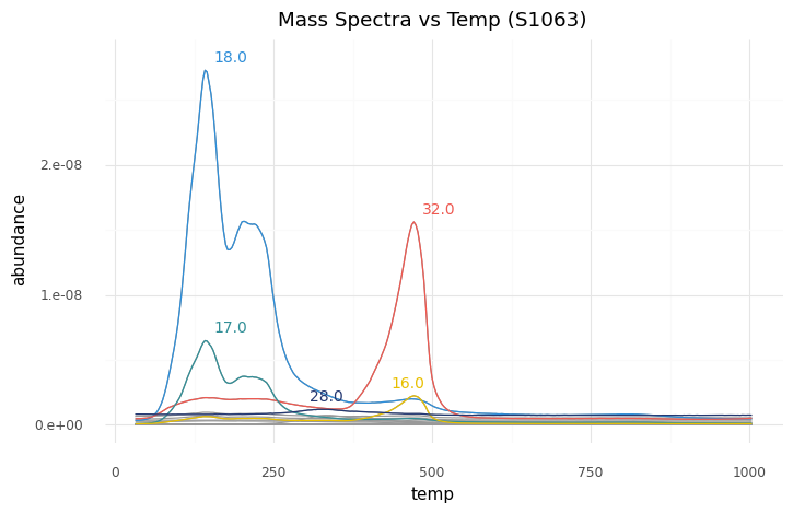
For example, the first-place winner's model took the data on the left, which was from a sample that contained iron oxide, oxychlorine, and phyllosilicate, to generate the predictions on the right:
| basalt | 0.008567 |
| carbonate | 0.006417 |
| chloride | 0.010731 |
| iron_oxide | 0.940646 |
| oxalate | 0.003044 |
| oxychlorine | 0.996400 |
| phyllosilicate | 0.991668 |
| silicate | 0.010867 |
| sulfate | 0.008285 |
| sulfide | 0.004359 |
| Note: compounds in blue were present in the sample. |
As with any research dataset like this one, initial algorithms may pick up on correlations that are incidental to the task. Our winners were able to discern real trends driven by the chemical signatures of these compounds, and one of our overall best performers also won the bonus prize for best performance and potential for future implementation for analysis of a smaller, noisier subset of the data. This subset, from the Sample Analysis at Mars (SAM) testbed, more closely resembles samples that are collected by the Curiosity rover directly from the surface of Mars.
Improving methods for analyzing planetary data helps scientists more quickly and effectively conduct mission operations and maximize scientific learnings as they move toward this ideal.

The NASA Mars Curiosity rover.
Results
Over the course of the competition, participants tested over 600 solutions and were able to contribute powerful models to the analysis of rock and soil samples using mass spectrometry. To kick off the competition, DrivenData released a benchmark solution that used a simple logistic regression model.
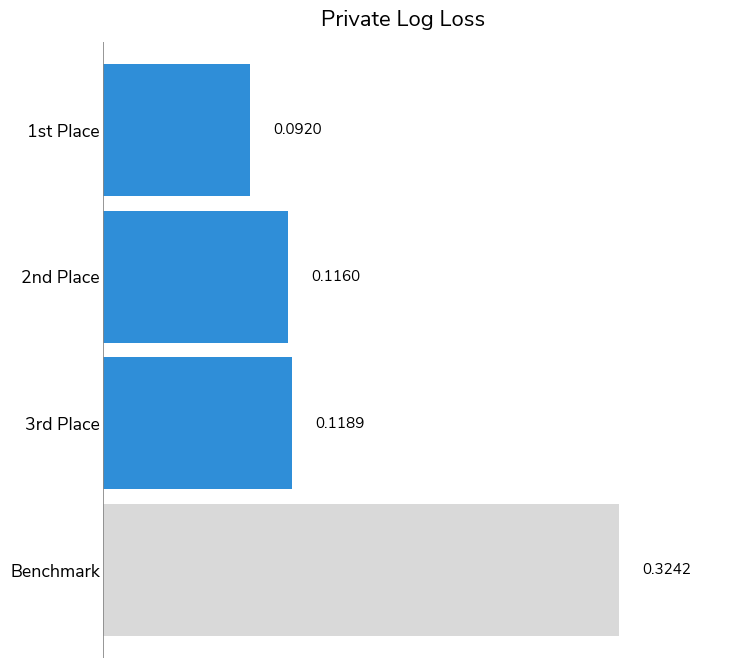
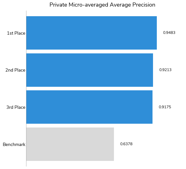
Overall, participants far outperformed the benchmark solution, with 446 out of 656 submissions besting the benchmark score. The log-loss established by the benchmark was 0.324 across all 10 compounds; our top performers achieved log-loss scores of 0.092, 0.116, and 0.119. We also took a look at the winning solutions' micro-averaged Average Precision (a.k.a. area under precision–recall curve). Average precision ranges from 0 to 1 (with 1 meaning perfect prediction) and measures how well models rank correct positive identifications with higher confidence than negative identifications. All three winners had strong average precision scores: 0.9483, 0.9213, 0.9175, respectively.
Competitors had a unique challenge when it came to the data on which their performance would be evaluated. Although most of the planetary soil analysis data available to scientists and our competitors is from commercial testbeds, which is cleaner, the ultimate goal of this mass spectrometry analysis is to produce a model that can perform as well on planetary soil sample data, which is scarcer and noisier. Therefore, a small portion of the training dataset contained samples from the SAM tested, a replica of the Sample Analysis at Mars (SAM) instrument suite onboard the Curiosity rover.
The test set contained more samples from the SAM testbed than the training set, which made it especially important for competitors to avoid overfitting and find ways to generalize in order to achieve a good score. The bonus prize was awarded by a judging panel of subject matter experts, who reviewed solution write-ups by the five competitors who performed best on the SAM testbed data for technical merit and potential for application to future data.
To achieve these results, the winners brought a wide variety of creative strategies to this task! Below are a few common approaches across solutions.
-
Feature engineering vs. neural network feature learning: The top performing solutions saw approaches that included both extensive feature engineering to capture the ion abundance curves and deep learning models that used image or sequence representations of the data as inputs. The first-place winner converted each mass spectrogram as a 2D image (temperature vs. m/z values) and did not perform any feature engineering. The third-place winner engineered features for the maximum temperature at the highest abundance, temperature range, and top 10 abundance values, among others. The second-place winner used both approaches in their ensemble of models—their solution included 1D convolutional networks as well as models with engineered features for area under the curve, peak value, peak-to-average, peak temperatures, width of peak, jitter, and then various statistics on the top three peaks.
-
Augmentation: The first-place winner made extensive use of augmentation, representing a single sample 16 times.
-
Ensembling: All of the winning solutions used some form of ensembling. Many trained multiple models with different types of preprocessing steps, model architectures, and deep learning model backbones. Some solutions also trained models on different subsets, or "folds", of the data. Ensembling, particularly with folds, can help avoid overfitting a model on the training data.
Encore!
Solutions in this challenge are intended to serve as a starting point for continued research and development. In fact, the challenge organizers will be launching a competition involving gas chromatography–mass spectrometry (GC–MS)—another method of chemical analysis that is used by the Curiosity rover's SAM instrument suite. Additionally, challenge organizers intend to make data from this challenge available online after the competition for ongoing improvement. Stay tuned for more in the coming weeks!
Now, let's get to know our winners and how they created such successful chemical analysis models! You can also dive into their open source solutions in the competition winners repo on Github.
Meet the winners
| Prize | Name |
|---|---|
| 1st place | Dmytro Poplavskiy |
| 2nd place | David Lander |
| 3rd place | Nikhil Mishra |
| Bonus | Dmytro Poplavskiy |
Dmytro Poplavskiy
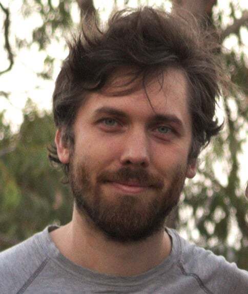
Place: 1st Place
Prize: $15,000
Hometown: Brisbane, Australia
Username: dmytro
Background:
My background is in software engineering, with an interest in Machine Learning. I do enjoy participating in machine learning challenges, I have won a number of competitions in the past.
What motivated you to compete in this challenge?
It's an interesting and unusual task, a new domain for me. It's a very exciting domain, not every day you can do something which may be used for Mars exploration!
Summary of approach:
I represented the mass spectrogram as a 2D image (temperature vs m/z values) used as an input to CNN, RNN or transformer-based models. The diverse set of preprocessing configurations and models helped to achieve the diverse ensemble of models.
A. David Lander

Place: 2nd Place
Prize: $7,500
Location: United States
Username: _NQ_
Background:
Winner of the M5 Uncertainty Forecasting Competition, Kaggle Coronavirus Forecasting Series, and U.S. Department of Justice Recidivism Forecasting Challenge (and previously #6 overall on Kaggle).
What motivated you to compete in this challenge?
I have a very strong background in time-series forecasting, and was looking to add signal processing experience.
Summary of approach:
The best performing architecture was a neural network with 2 Conv1d modules, operating over temperature, followed by a Linear layer across m/z channels and then a multi-target classifier.
The network inputs are the first 100 m/z channels, with temperature binned into 25 degree increments. Temperatures included are roughly 100 to 1100 degrees, with random noise applied to produce a diverse set of models.
All Conv1d modules are kernel 3, stride 2, and the first layer involves dilations of 1, 2, 5, 10, 20, 50, and 100, with zero padding. All blocks use Group Normalization, Dropout (about 0.1), and Random ReLU (about 1/3 to 1/8 negative slope), with final layer dropout of 0.5.
Three different input scalings are used: - divide by sum of all m/z values at a given temperature (best) - divide by sum of all temperature values for a given m/z taken to the 0.5 - 1.0 power (second best) - divide by the maximum value across the entire array (third best)
Models include either the first, first and second, or all three channels, with substantial gains from ensembling all three approaches.
All models were trained for up to 100 epochs with SGDP without momentum at a learning rate of 0.1 and a batch size of 12.
What are some other things you tried that didn’t necessarily make it into the final workflow?
Replacing the Linear layer aggregating across m/z with a Transformer would be a good first place to start, as there are clear relationships between ions. Improving performance on SAM samples is also possible with a CycleGAN model that translates between SAM spectra and commercial spectra (these were distinguishable with 100% accuracy).
Nikhil Kumar Mishra
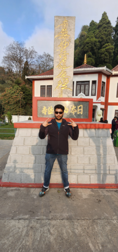
Place: 3rd Place
Prize: $5,000
Hometown: Siliguri, West Bengal State, India
Username: devnikhilmishra
Background:
Hi, I am Nikhil Kumar Mishra, currently working as a Data Scientist for Okcredit, a startup in Bangalore.
What motivated you to compete in this challenge?
I loved participating in Data Science competitions, since the time I started to learn Data Science, and am always on the lookout for something interesting. I am also fortunate to have finished top 3 in many of them. I think I had never worked seriously on signal data before, so this challenge was a perfect way to hone my skills. Also a competition hosted by NASA on drivendata would surely bring a lot of amazing participants, so I could not pass this opportunity.
Summary of approach:
I converted the multilabel problem into a binary classification problem. Given a combination of a sample_features + compound, tell if the compound is present in the sample. For a given sample, features were the same for each compound, except the feature telling which compound we were predicting. I used lightgbm k fold ensemble model to get the initial predictions, then fed these predictions along with top 5k features to a 31 fold ensemble, catboost model (which acted like a meta model). 2 stage modelling helped quite a lot in this competition, because the presence of one compound could help in the determination of others. Number of folds were high because I felt the data was quite small, so I wanted to have most of the samples in training. I will describe the thought process behind feature-engineering now, as it was very crucial in this competition.
Almost all my feature engineering was done per m/z instead of per sample_id.
I pre-sorted each sample_id’s data mass spectra by abundance in descending order, to help with feature creation, since signal characteristics near the peak were strong indicators of presence of compounds.
I saw was the signals were quite noisy specially from SAM test-bed, so I tried to smoothen the signals and convert them to fix length per m/z, per sample_id, so I could have fixed length features for each sample_id, this alone gave me a lot of boost in my score. After some trial and error I stuck to 25 length sequence, and created features for abundance and temperature using that, both with sorted by abundance and by their original time order
I followed the following steps, to get aggregation features per m/z, sorting the data in abundance descending order. (Please refer to the code too, as it might be tricky to read)
- Firstly, create a list of values of k which basically tells to get top k values for each sample. Since all sample_ids had different length mass spectra, I normalized the length of each of the spectra, and then took top k% of the samples. k had values starting from 0.001 (top 0.1% of the values) to 0.2 (top 20%).
- Create features by aggregating abundance (normalized frequency, mean, standard_deviation) per m/z and temp_bin (temperature was binned per sample_id into 5 buckets)
- Create features by aggregating temperature and abundance per m/z.
- For features created in 2 and 3, I took the ratio of the features generated by current k, to the features generated by previous k.
- I also created sample level features, like max_temperature at highest abundance, range of temperature and top 10 abundance values, etc.
- Finally I created features by aggregating temp on m/z and abundance_bin (I binned abundance of each sample_id into 8 equal parts) for all the values (not top k values).
My general approach to feature engineering and modelling is to add a feature and keep it only if it helps in the model evaluation, and remove it if it doesn't improve the evaluation, feature generation and evaluation of the model must be done together.
Bonus prize
Performance on samples from the SAM testbed are of significant interest to NASA scientists, since the data collected from the testbed is meant to replicate the SAM instrument suite on Curiosity on Mars, and will also more closely resemble the data that would be collected by future Mars missions. The top five participants ranked by their performance on the SAM testbed samples were invited to submit a brief write-up of their methodology for review by a panel of subject matter experts. Based on both his performance on the SAM testbed data and the potential of his approach, our first-place winner dmytro won the bonus prize as well. You can read more about his solution below and find his full bonus prize write-up here.
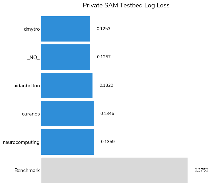
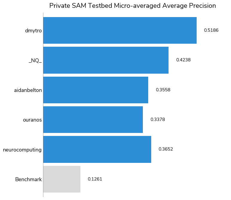
The task of making correct predictions for the SAM testbed data is clearly more difficult than for the overall dataset, as evidenced by the higher overall log-loss scores and the lower overall Micro-averaged Average Precision (MAP). While the highest MAP was 0.9483 for the overall test set, it was 0.5186 for the SAM testbed subset.
Bonus prize winner: Dmytro Poplavskiy

Place: Bonus prize: SAM testbed modeling methodology
Prize: $2,500
Username: dmytro
Summary of approach to SAM testbed data:
Overall the solution does not rely as much on pre- and postprocessing of the SAM testbed as on augmentation of the commercial data. The only difference in preprocessing for the SAM testbed data is that because the data looks noisier, the SAM testbed samples are averaged over 4-degree bins.
To avoid overfitting to the training dataset and make the models more generalisable to the SAM testbed samples, the following augmentations have been applied during training and prediction:
- Randomly choose to correct for background, either subtract the estimated baseline or simply a minimum value. In both cases, the random combination of 0.1%, 5%, 10% and 20% percentiles is subtracted.
- Random query of the abundance values from the overlapping temperature bands when converting to 2D image.
- Every m/z plot is randomly scaled by 2 random_normal(0 mean, sigma) with 1.0 or 0.5 sigma values.
- For some models, instead of normalizing data by maximum value over all measurements, m/z plots are normalized to 1 individually. Surprisingly, the models' performance was similar to the maximum scaling. So some models in the ensemble were trained with the max normalization and some with per m/z band normalization.
- Mixing two samples. 2D representations of two samples are mixed together, either as an average or maximum value with the label combined as maximum. Mixing a few available SAM testbed samples with commercial samples may help to generalize to other SAM testbed samples.
If you were to continue working on this problem for the next year, what methods or techniques might you try in order to build on your work so far?
With only 12 SAM testbed samples available for training and validation, and given such a drastic difference between the commercial and the SAM testbed data, I don’t really expect the model to perform very well. Collecting more training samples is the most obvious and straightforward way to improve the model performaxsnce, but since the number of the SAM testbed samples is limited, just adding them to the training set is not the most efficient way. It may work better to use the extra samples and understanding of processes that caused the difference with the commercial data, to design the better augmentations processes (for example to generate the random background, similar to possible SAM testbed cases). Mixing the small number of the SAM testbed samples with a large number of available commercial data should also work as a very good augmentation technique.
Other bonus prize finalists
Our other bonus prize finalists were _NQ_, aidanbelton, ouranos, and neurocomputing. Thank you to these finalists for submitting their write-ups for review! As with the overall competition finalists, there were some common approaches used by the bonus prize finalists:
-
Ensembling: All five bonus prize finalists ensembled several models together in order to arrive upon their final predictions.
-
Both deep learning and gradient-boosted trees: Multilayer perceptrons and LightGBM models were the two most common architectures across many of the finalists. 2D image models and RNNs also saw some use across multiple finalists.
-
Preprocessing: Finalists experimented with preprocessing steps, feature engineering on characterizing peaks, and data augmentation.
Thanks to all the participants and to our winners! Special thanks to NASA for enabling this fascinating challenge and providing the data to make it possible!


