Welcome to the benchmark notebook for Mars Spectrometry: Detect Evidence for Past Habitability! The problem description for this challenge can be found here. The purpose of this notebook is to provide an example of how to use the data to create a basic benchmark model and to demonstrate how to submit your work.
Did Mars ever have livable environmental conditions? This is one of the key questions in the field of planetary science. NASA missions like the Curiosity and Perseverance rovers carry a rich array of scientific instruments to collect data that can help answer this question, including instruments that gather and analyze rock and soil samples. Using a method of chemical analysis called evolved gas analysis (EGA), the samples can be analyzed for their chemical makeup, which can indicate whether the environment's conditions could have been amenable to life.
In this challenge, your goal is to build a model to automatically analyze EGA mass spectrometry data to detect the presence of ten families of chemical compounds related to understanding Mars' potential for past habitability.
The winning techniques from this competition may be used to help analyze data from Mars, and potentially even inform future designs for planetary mission instruments performing in-situ analysis. In other words, one day your model might literally be out-of-this-world!
In this notebook, we'll cover:
- Exploratory data analysis
- Preprocessing
- Feature engineering
- Training a logistic regression model
- Preparing a submission
Let's get started!
import itertools
from pathlib import Path
from pprint import pprint

from matplotlib import pyplot as plt, cm
import numpy as np
import pandas as pd
from pandas_path import path
from sklearn.dummy import DummyClassifier
from sklearn.preprocessing import minmax_scale
from sklearn.linear_model import LogisticRegression
from sklearn.metrics import make_scorer, log_loss
from sklearn.model_selection import StratifiedKFold, cross_val_score
from tqdm import tqdm

pd.set_option("max_colwidth", 80)
RANDOM_SEED = 42  # For reproducibility
Importing datasets
In this competition, there are three datasets:
- the training set, for which both features and labels are provided;
- the validation set, for which you will submit predictions, and your score will be displayed on the leaderboard while the competition is open
- the test set, for which you will also submit predictions, and your score will be used in determining the final rankings
This competition also has two phases: an initial development phase for the first half and a final training phase for the second half. In the second phase, the labels for the validation set will be released so that the validation set can be used as additional training data.
We will therefore perform light exploratory data analysis on the data available to us at the beginning of the competition - the features and labels for the training set, and the features for the validation and test sets. metadata.csv contains information about each sample included in the dataset, including whether it's a part of training, validation, or testing dataset and which instrument the data was collected by.
DATA_PATH = Path.cwd().parent / "data/final/public/"
metadata = pd.read_csv(DATA_PATH / "metadata.csv", index_col="sample_id")
metadata.head()
train_files = metadata[metadata["split"] == "train"]["features_path"].to_dict()
val_files = metadata[metadata["split"] == "val"]["features_path"].to_dict()
test_files = metadata[metadata["split"] == "test"]["features_path"].to_dict()

print("Number of training samples: ", len(train_files))
print("Number of validation samples: ", len(val_files))
print("Number of testing samples: ", len(test_files))
Exploratory data analysis
The data for this competition is composed of evolved gas analysis mass spectrograms from two different types of instruments: commercial instruments, and the Sample Analysis at Mars (SAM) testbed. Data from these two instruments differ in many ways, as detailed in the relevant section of the Problem Description page. As we explore the dataset, we will highlight some of the differences.
First, let's see what proportion of samples in the training, validation, and test set are composed of each instrument type.
# Share of samples from commercial instruments vs. SAM testbed
meta_instrument = (
    metadata.reset_index()
    .groupby(["split", "instrument_type"])["sample_id"]
    .aggregate("count")
    .reset_index()
)
meta_instrument = meta_instrument.pivot(
    index="split", columns="instrument_type", values="sample_id"
).reset_index()
meta_instrument.head()

ax = meta_instrument.plot(
    x="split",
    kind="barh",
    stacked=True,
    title="Instrument type by dataset split",
    mark_right=True,
)
ax.bar_label(ax.containers[0], label_type="center")
ax.bar_label(ax.containers[1], label_type="center")

We can see that in general, there is a much greater share of commercial instrument samples in the competition data. Furthermore, there are very few SAM testbed samples in training set, and none at all in the validation set. In this competition, it is expected that modeling the SAM testbed data will be difficult, and that there will need to be transfer learning from the commercial instrument data in order to successfully model the SAM testbed data.
Note that the competition has a bonus prize associated with modeling the SAM testbed samples specifically. The top performers on the SAM testbed samples within the test set will be invited to submit a report of their methodology, to be judged by a panel of experts from NASA. See the Timeline and Prizes information for the competition for more details.
Let's look at the distribution of various compounds of interest in our training data.
train_labels = pd.read_csv(DATA_PATH / "train_labels.csv", index_col="sample_id")
train_labels.head()
sumlabs = train_labels.aggregate("sum").sort_values()
plt.barh(sumlabs.index, sumlabs, align="center")
plt.ylabel("Compounds")
plt.xticks(rotation=45)
plt.xlabel("Count in training set")
plt.title("Compounds represented in training set")

We can use some plots to understand how a few different variables relate to each other. We have only four variables available to us - time, which is the time from the start of the experiment, temp, the temperature that the sample is heated to at that point in time, m/z, which is a "type" of ion detected, and abundance, which is the amount of the ion type detected at the temperature and point in time.
First, we can observe the relationship between temperature and time. Temperature is supposed to be a function of time in these experiments, but the patterns of ion abundance may vary as a function of both. Further, the commercial and testbed samples may contain a different range of times and temperatures, so let's examine a few samples of each type.
# Select sample IDs for five commercial samples and five testbed samples
sample_id_commercial = metadata[metadata["instrument_type"] == "commercial"].index.values[
    0:5
]
sample_id_testbed = metadata[metadata["instrument_type"] == "sam_testbed"].index.values[
    0:5
]
# Import sample files for EDA
sample_commercial_dict = {}
sample_testbed_dict = {}

for i in range(0, 5):
    comm_lab = sample_id_commercial[i]
    sample_commercial_dict[comm_lab] = pd.read_csv(DATA_PATH / train_files[comm_lab])

    test_lab = sample_id_testbed[i]
    sample_testbed_dict[test_lab] = pd.read_csv(DATA_PATH / train_files[test_lab])
# Plot time vs. temperature for both sample types

# For commercial
fig, ax = plt.subplots(1, 5, figsize=(15, 3), constrained_layout=True, sharey="all")
fig.supylabel("Temperature")
fig.supxlabel("Time")
fig.suptitle("Commercial samples")

for i in range(0, 5):
    sample_lab = sample_id_commercial[i]
    plt.subplot(1, 5, i + 1)
    plt.scatter(
        sample_commercial_dict[sample_lab]["time"],
        sample_commercial_dict[sample_lab]["temp"],
    )
    plt.title(sample_lab)

# For SAM testbed
fig, ax = plt.subplots(1, 5, figsize=(15, 3), constrained_layout=True, sharey="all")
fig.supylabel("Temperature")
fig.supxlabel("Time")
fig.suptitle("SAM testbed samples")

for i in range(0, 5):
    sample_lab = sample_id_testbed[i]
    plt.subplot(1, 5, i + 1)
    plt.scatter(
        sample_testbed_dict[sample_lab]["time"],
        sample_testbed_dict[sample_lab]["temp"],
    )
    plt.title(sample_lab)


In general, the samples have similar linear ramp-ups in temperature from around 0º to around 1,000º over a period of around 1,600 seconds. However, some samples are heated for less time and/or to a lower maximum temperature. Additionally, testbed samples more often have some non-linear heating profiles. These are differences you may wish to account for in our preprocessing steps. A simple approach may ignore the time dimension and only consider the ion abundances as a function of temperature. However, there may be nuances to how the sample was heated over time that provides additional information.
Let's also look at the two other key values - m/z, which indicates the type of an ion, and abundance, which indicates that ion type's levels across temperature and time. We can visualize changes in abundance across temperature and time, which can help us identify relationships within the data that chemists might consider when identifying compounds.
# For commercial
fig, ax = plt.subplots(1, 5, figsize=(15, 3), constrained_layout=True)
fig.suptitle("Commercial samples")
fig.supxlabel("Temperature")
fig.supylabel("Abundance")

for i in range(0, 5):
    sample_lab = sample_id_commercial[i]
    sample_df = sample_commercial_dict[sample_lab]

    plt.subplot(1, 5, i + 1)
    for m in sample_df["m/z"].unique():
        plt.plot(
            sample_df[sample_df["m/z"] == m]["temp"],
            sample_df[sample_df["m/z"] == m]["abundance"],
        )

    plt.title(sample_lab)

# For testbed
fig, ax = plt.subplots(1, 5, figsize=(15, 3), constrained_layout=True)
fig.suptitle("SAM testbed samples")
fig.supxlabel("Temperature")
fig.supylabel("Abundance")

for i in range(0, 5):
    sample_lab = sample_id_testbed[i]
    sample_df = sample_testbed_dict[sample_lab]

    plt.subplot(1, 5, i + 1)
    for m in sample_df["m/z"].unique():
        plt.plot(
            sample_df[sample_df["m/z"] == m]["temp"],
            sample_df[sample_df["m/z"] == m]["abundance"],
        )
    plt.title(sample_lab)


We can see from the above that there are different m/z ion types that peak at different temperatures. (Each colored line represents a distinct m/z value). However, we can see across most samples that there is one m/z ion that is consistently high in abundance throughout the run. While we don't label the lines with m/z for this overview visualization (there may be hundreds of lines), further digging would reveal that ion to be for m/z=4, which we know from the problem description is ions from helium carrier gas and is not from the sample itself. We can also see that for some samples, there are other ion types that are consistently present at low abundance levels - which are likely background abundances that are also irrelevant. (In general, a spectrogram is useful for the peaks in abundances it shows at different temperatures and times).
It seems that we'll need to do some preprocessing to make any trends clearer.
Preprocessing
From the "Understanding EGA–MS Data" section of the project description page, we know that there are several preprocessing steps that will likely be helpful before working with the data. We'll demonstrate each step on a single sample to visualize the changes.
# Selecting a testbed sample to demonstrate preprocessing steps
sample_lab = sample_id_testbed[1]
sample_df = sample_testbed_dict[sample_lab]
1. Standardizing which m/z values to include
As described in the problem description page, there is some heterogeneity in the m/z values measured for each sample. In this section, we will make some basic simplifying assumptions to standardize which m/z values to include in our analysis.
As you will see, the range of m/z values being measured is not the same for every sample. Because most samples have m/z from 0 to 99, we will discard any m/z values above 99. Additionally, the SAM testbed samples contain fractional m/z values, but as the problem description page discusses, these abundances are highly correlated with the closest whole number values. Therefore, we will also drop these fractional m/z values.
Additionally, as discussed on the problem description page, samples may have a high level of ions for m/z=4.0, which corresponds to helium carrier gas. The helium is not relevant to the composition of the sample, so we will also discard it as simplification. A more sophisticated analysis could potentially use it to understand how other ions compare to it relatively.
def drop_frac_and_He(df):
    """
    Drops fractional m/z values, m/z values > 100, and carrier gas m/z

    Args:
        df: a dataframe representing a single sample, containing m/z values

    Returns:
        The dataframe without fractional an carrier gas m/z
    """

    # drop fractional m/z values
    df = df[df["m/z"].transform(round) == df["m/z"]]
    assert df["m/z"].apply(float.is_integer).all(), "not all m/z are integers"

    # drop m/z values greater than 99
    df = df[df["m/z"] < 100]

    # drop carrier gas
    df = df[df["m/z"] != 4]

    return df
# m/z values before limiting
fig, ax = plt.subplots(1, 2, figsize=(10, 5))
fig.suptitle("Distribution of m/z values")
fig.supxlabel("m/z")
fig.supylabel("Count of observations")

plt.subplot(1, 2, 1)
plt.hist(sample_df["m/z"])
plt.title("Before dropping selected m/z values")

# m/z values after limiting
sample_df = drop_frac_and_He(sample_df)
plt.subplot(1, 2, 2)
plt.hist(sample_df["m/z"])
plt.title("After dropping selected m/z values")

2. Removing background ion presences
As discussed in the problem description, there will be background levels of ions in the measurements that aren't relevant to the analysis. While there are more complex and nuanced ways to remove the background noise, we will simply subtract the minimum abundance value. As mentioned in the project description, scientists may remove background noise more carefully. They may take an average of an area early in the experiment to subtract. Or, if the background noise varies over time, they may fit a function to it and subtract according to this function.
def remove_background_abundance(df):
    """
    Subtracts minimum abundance value

    Args:
        df: dataframe with 'm/z' and 'abundance' columns

    Returns:
        dataframe with minimum abundance subtracted for all observations
    """

    df["abundance_minsub"] = df.groupby(["m/z"])["abundance"].transform(
        lambda x: (x - x.min())
    )

    return df
# Abundance values before subtracting minimum
fig, ax = plt.subplots(1, 2, figsize=(15, 5))
fig.suptitle("Abundance values across temperature by m/z")
fig.supxlabel("Temperature")
fig.supylabel("Abundance levels")

plt.subplot(1, 2, 1)
for m in sample_df["m/z"].unique():
    plt.plot(
        sample_df[sample_df["m/z"] == m]["temp"],
        sample_df[sample_df["m/z"] == m]["abundance"],
    )
plt.title("Before subtracting minimum abundance")

# After subtracting minimum abundance value
sample_df = remove_background_abundance(sample_df)

plt.subplot(1, 2, 2)
for m in sample_df["m/z"].unique():
    plt.plot(
        sample_df[sample_df["m/z"] == m]["temp"],
        sample_df[sample_df["m/z"] == m]["abundance_minsub"],
    )
plt.title("After subtracting minimum abundance")

3. Convert abundances to relative abundances
Since the relative abundances of various ions are more informative than their absolute values, we normalize the abundance values from 0 to 1 within a single sample.
def scale_abun(df):
    """
    Scale abundance from 0-100 according to the min and max values across entire sample

    Args:
        df: dataframe containing abundances and m/z

    Returns:
        dataframe with additional column of scaled abundances
    """

    df["abun_minsub_scaled"] = minmax_scale(df["abundance_minsub"].astype(float))

    return df
Putting it all together
Finally, let's revisit what our samples look like after all of the preprocessing steps have been completed.
# Preprocess function
def preprocess_sample(df):
    df = drop_frac_and_He(df)
    df = remove_background_abundance(df)
    df = scale_abun(df)
    return df
# For commercial
fig, ax = plt.subplots(1, 5, figsize=(15, 3), constrained_layout=True)
fig.suptitle("Commercial samples")
fig.supxlabel("Temperature")
fig.supylabel("Abundance")

for i in range(0, 5):
    sample_lab = sample_id_commercial[i]
    sample_df = sample_commercial_dict[sample_lab]
    sample_df = preprocess_sample(sample_df)

    plt.subplot(1, 5, i + 1)
    for m in sample_df["m/z"].unique():
        plt.plot(
            sample_df[sample_df["m/z"] == m]["temp"],
            sample_df[sample_df["m/z"] == m]["abun_minsub_scaled"],
        )

    plt.title(sample_lab)

# For testbed
fig, ax = plt.subplots(1, 5, figsize=(15, 3), constrained_layout=True)
fig.suptitle("SAM testbed samples")
fig.supxlabel("Temperature")
fig.supylabel("Abundance")

for i in range(0, 5):
    sample_lab = sample_id_testbed[i]
    sample_df = sample_testbed_dict[sample_lab]
    sample_df = preprocess_sample(sample_df)

    plt.subplot(1, 5, i + 1)
    for m in sample_df["m/z"].unique():
        plt.plot(
            sample_df[sample_df["m/z"] == m]["temp"],
            sample_df[sample_df["m/z"] == m]["abun_minsub_scaled"],
        )
    plt.title(sample_lab)


After preprocessing, the peaks in our data for different m/z values are more apparent.
Feature engineering
When scientists analyze EGA data, they look closely at the characteristics of peaks in ion abundances, such as the temperatures at which they occur, the shape of the peaks including height, width, and area. For our analysis, we will engineer a simple set of features that try to capture some of these characteristics. We will discretize the overall temperature range into bins (of 100 degrees), and calculate maximum relative abundance within that temperature bin for each m/z value.
There are many ways to describe the shapes of these peaks with higher fidelity than the approach we demonstrate here. It will also be important to deal with complex cases such as peaks that overlap due to two different gas releases producing the same ions at around the same time. We look forward to seeing what you all come up with in your own feature engineering.
# Create a series of temperature bins
temprange = pd.interval_range(start=-100, end=1500, freq=100)
temprange

# Make dataframe with rows that are combinations of all temperature bins
# and all m/z values
allcombs = list(itertools.product(temprange, [*range(0, 100)]))

allcombs_df = pd.DataFrame(allcombs, columns=["temp_bin", "m/z"])
allcombs_df.head()
def abun_per_tempbin(df):
    """
    Transforms dataset to take the preprocessed max abundance for each
    temperature range for each m/z value

    Args:
        df: dataframe to transform

    Returns:
        transformed dataframe
    """

    # Bin temperatures
    df["temp_bin"] = pd.cut(df["temp"], bins=temprange)

    # Combine with a list of all temp bin-m/z value combinations
    df = pd.merge(allcombs_df, df, on=["temp_bin", "m/z"], how="left")

    # Aggregate to temperature bin level to find max
    df = df.groupby(["temp_bin", "m/z"]).max("abun_minsub_scaled").reset_index()

    # Fill in 0 for abundance values without information
    df = df.replace(np.nan, 0)

    # Reshape so each row is a single sample
    df = df.pivot_table(columns=["m/z", "temp_bin"], values=["abun_minsub_scaled"])

    return df
# Assembling preprocessed and transformed training set

train_features_dict = {}
print("Total number of train files: ", len(train_files))

for i, (sample_id, filepath) in enumerate(tqdm(train_files.items())):
    # Load training sample
    temp = pd.read_csv(DATA_PATH / filepath)

    # Preprocessing training sample
    train_sample_pp = preprocess_sample(temp)

    # Feature engineering
    train_sample_fe = abun_per_tempbin(train_sample_pp).reset_index(drop=True)
    train_features_dict[sample_id] = train_sample_fe

train_features = pd.concat(
    train_features_dict, names=["sample_id", "dummy_index"]
).reset_index(level="dummy_index", drop=True)
train_features.head()
# Make sure that all sample IDs in features and labels are identical
assert train_features.index.equals(train_labels.index)
Perform modeling
This competition's task is a multi-label classification problem with 10 label classes—each observation can belong to any number of the label classes. One simple modeling approach for multi-label classification is "one vs. all", in which we create a binary classifier for each label class independently. Then, each binary classifier's predictions are simply concatenated together at the end for the overall prediction. For this benchmark, we will use logistic regression for each classifier as a first-pass modeling approach.
In order to have a reference point for our model, it can help to have a naive baseline. This challenge's metric is aggregated log-loss. Log-loss has the property that it is optimized by statistically calibrated predicted probabilities. Therefore, a good baseline model to use is to predict the proportion of each label class in the training set.
We will also use K-fold cross-validation to evaluate our model, rather than just a simple train-test split. K-fold cross-validation makes use of all of the data we have available for training and evaluation and is a useful technique for cases of having a relatively small amount of labeled data. When generating the cross-validation folds, we will also stratify according to class to make sure that there is even representation of each class for each fold. We will set a random seed in order to use the same cross-validation folds for both the dummy baseline model and the logistic regression model for an apples-to-apples comparison.
# Define stratified k-fold validation
skf = StratifiedKFold(n_splits=10, random_state=RANDOM_SEED, shuffle=True)

# Define log loss
log_loss_scorer = make_scorer(log_loss, needs_proba=True)
Baseline dummy classifier
# Check log loss score for baseline dummy model
def logloss_cross_val(clf, X, y):
    # Generate a score for each label class
    log_loss_cv = {}
    for col in y.columns:
        y_col = y[col]  # take one label at a time
        log_loss_cv[col] = np.mean(
            cross_val_score(clf, X.values, y_col, cv=skf, scoring=log_loss_scorer)
        )

    avg_log_loss = np.mean(list(log_loss_cv.values()))

    return log_loss_cv, avg_log_loss
# Dummy classifier
dummy_clf = DummyClassifier(strategy="prior")

print("Dummy model log-loss:")
dummy_logloss = logloss_cross_val(dummy_clf, train_features, train_labels)
pprint(dummy_logloss[0])
print("\nAverage log-loss")
dummy_logloss[1]
Now that we have a log-loss value from a very naive approach, we have a baseline against which to compare the performance of future approaches.
Logistic regression model
For our logistic regression models, we will also use lasso (a.k.a. L1) regularization, which will reduce the number of features used in the prediction. This will be helpful for the much greater number of features (1600) than observations. More sophisticated dimensionality reduction techniques, such as principal component analysis (PCA), may be useful, but we will just stick with a simple approach for this benchmark.
We've found that a regularization weight parameter of C=10 seems to work okay. To further tune this model, we would recommend using a cross-validated hyperparameter optimizer.
# Define logistic regression model
logreg_clf = LogisticRegression(
    penalty="l1", solver="liblinear", C=10, random_state=RANDOM_SEED
)
print("Logistic regression model log-loss:\n")
logreg_logloss = logloss_cross_val(logreg_clf, train_features, train_labels)
pprint(logreg_logloss[0])
print("Average log-loss")
logreg_logloss[1]
Training the model on all of the data
Now that we've used cross-validation to get an idea of our performance, we want to use all of the training data to train our model.
# Train logistic regression model with l1 regularization, where C = 10

# Initialize dict to hold fitted models
fitted_logreg_dict = {}

# Split into binary classifier for each class
for col in train_labels.columns:
    y_train_col = train_labels[col]  # Train on one class at a time

    # output the trained model, bind this to a var, then use as input
    # to prediction function
    clf = LogisticRegression(
        penalty="l1", solver="liblinear", C=10, random_state=RANDOM_SEED
    )
    fitted_logreg_dict[col] = clf.fit(train_features.values, y_train_col)  # Train
# Create dict with both validation and test sample IDs and paths
all_test_files = val_files.copy()
all_test_files.update(test_files)
print("Total test files: ", len(all_test_files))
# Import submission format
submission_template_df = pd.read_csv(
    DATA_PATH / "submission_format.csv", index_col="sample_id"
)
compounds_order = submission_template_df.columns
sample_order = submission_template_df.index
def predict_for_sample(sample_id, fitted_model_dict):
    # Import sample
    temp_sample = pd.read_csv(DATA_PATH / all_test_files[sample_id])

    # Preprocess sample
    temp_sample = preprocess_sample(temp_sample)

    # Feature engineering on sample
    temp_sample = abun_per_tempbin(temp_sample)

    # Generate predictions for each class
    temp_sample_preds_dict = {}

    for compound in compounds_order:
        clf = fitted_model_dict[compound]
        temp_sample_preds_dict[compound] = clf.predict_proba(temp_sample.values)[:, 1][0]

    return temp_sample_preds_dict
# Dataframe to store submissions in
final_submission_df = pd.DataFrame(
    [
        predict_for_sample(sample_id, fitted_logreg_dict)
        for sample_id in tqdm(sample_order)
    ],
    index=sample_order,
)
final_submission_df.head()
# Check that columns and rows are the same between final submission and submission format
assert final_submission_df.index.equals(submission_template_df.index)
assert final_submission_df.columns.equals(submission_template_df.columns)
The shape and layout of our prediction dataframe looks good! Each row is a unique sample and each column corresponds to a class. We will now generate a csv and submit.
final_submission_df.to_csv("benchmark_logreg_submission.csv")
Upload submission
We can now head over to the competition submissions page to submit our predictions and see how we score! Click on "Make new submission" and upload your formatted prediction CSV file.

Our model got a 0.2733 on the validation set. Not a bad start! Both the logistic regression model and our previous baseline dummy model (named as "Training Set Prior Distributions") have been added to competition leaderboard as benchmarks.
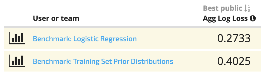
We can see that our logistic regression model is doing better than the baseline. Now it's up to you to improve on it!
Good luck!
We hope this benchmark solution provided a helpful framework for getting started. Head over to the Mars Spectrometry: Detect Evidence for Past Habitability homepage for more details on the competition, and you can also check out the forum. We can't wait to see what you build!
Image of Curiosity courtesy of NASA/JPL-Caltech/MSSS.