The Challenge
Exposure to air pollution is the top environmental risk factor for premature death, but millions of people across the globe don't have access to reliable data about their current local air quality.
Algorithms that combine data from satellites with data from ground monitors are critical to filling this information gap. Insights from this challenge will be shared as broadly as possible to help advance the field and ultimately allow everyone to better protect themselves from air pollution.
Abbey Nastan, MAIA Deputy Program Applications Lead, NASA's Jet Propulsion Laboratory in Southern California
Motivation
Air pollution is one of the greatest environmental threats to human health. It can result in heart and chronic respiratory illness, cancer, and premature death. Currently, no single satellite instrument provides ready-to-use, high resolution information on surface-level air pollutants. This gap in information means that millions of people cannot take daily action to protect their health.
The goal of this challenge was to use remote sensing data and other geospatial data sources to develop models for estimating daily levels of air pollution with high spatial resolution. This competition focused on two critical air quality measures:
- Particulate matter less than 2.5 micrometers in size (PM2.5) can last days to weeks in the atmosphere and penetrate deep into human lungs, increasing the risk of heart disease, lower respiratory infections, and poor pregnancy outcomes.
- Nitrogen Dioxide (NO2) forms in the atmosphere from the burning of fossil fuels such as coal, oil, or gas, and has a short lifetime on the order of hours near the surface. It can cause respiratory issues, while also contributing to the production of ozone and nitrate aerosols, a component of PM2.5.
Participants competed separately in two different tracks - Particulate Matter (PM2.5) and Trace Gas (NO2).

Air pollution includes gases (e.g. NO2) and particles (e.g. PM2.5). Source: NASA JPL
Data Overview
Existing high-quality ground monitors measure PM2.5 and NO2, but are expensive and have large gaps in coverage. Models that make use of widely available satellite data have the potential to provide local, daily air quality information.
This challenge was set-up using measurements from reference-grade monitors pulled from OpenAQ as ground-truth. Data derived from satellite instruments were used as input. Models were tasked with predicting surface-level PM2.5 and NO2 levels in micrograms per cubic meter (µg/m³) with:
- high-resolution (5km by 5km grid cells)
- high frequency (daily)
- geographic diversity - Los Angeles (South Coast Air Basin), Delhi, and Taipei. These locations represent areas with readily available satellite data, but varying levels of pollution and historical data.
Satellite data
In the Particulate Matter Track, the primary measure that is useful for predicting pollutant levels is Aerosol Optical Depth (AOD), a unitless measure of aerosols distributed within a column of air from Earth's surface to the top of the atmosphere. Competitors were required to use one of two critical sources of AOD measurements:
- Multi-angle Implementation of Atmospheric Correction (MAIAC) is an algorithm that combines pixel- and image-based processing to improve the accuracy of the aerosol, cloud, and atmospheric data retrieved from MODIS, a key instrument aboard NASA's Terra and Aqua satellites.
- Multi-angle Imaging SpectroRadiometer (MISR) is an instrument, also aboard the Terra satellite, that is collecting important data on the causes and effects of global climate change.
In the Trace Gas Track, the primary measurement is NO2 vertical column density (NO2 VCD). Competitors were required to use one of two critical data sources:
- The Ozone Monitoring Instrument (OMI) aboard NASA's Aura satellite measures criteria pollutants such as O3, NO2, SO2, and aerosols from Earth's surface to top-of-atmosphere.
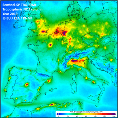
- The TROPOspheric Monitoring Instrument (TROPOMI) is on board the Copernicus Sentinel-5 Precursor satellite. This product contains Total column NO2 and Tropospheric Column NO2, for all atmospheric conditions, and for sky conditions where cloud fraction is less than 30 percent.

|
|
| Above: Combined MODIS Optical Depth 047 data from the MCD19A2 product over part of west Africa, June 3, 2018. Source: USGS | Above: TROPOMI tropospheric NO2 column data visualized of Europe in 2019. Source: EU, ESA, KNMI |
Results
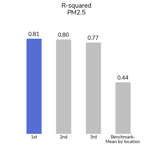
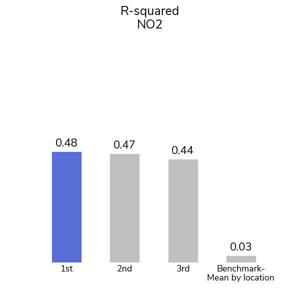
Participants were able to see the pattern through the pollution with more than 1,200 submissions from over 1,000 participants over the course of the competition! The top model for the PM2.5 track achieved an R-squared value of 0.81 and the top model for the NO2 track achieved an R-squared value of 0.48.
To help participants get started, a blog post was published for each track the demonstrate how to work with and derive features from the satellite data. A simple random forest model was trained only on data from LA using basic summary statistics as features. The PM2.5 benchmark achieved an R-squared on the public leaderboard of -0.07, while the NO2 benchmark achieved an R-squared of -0.15.
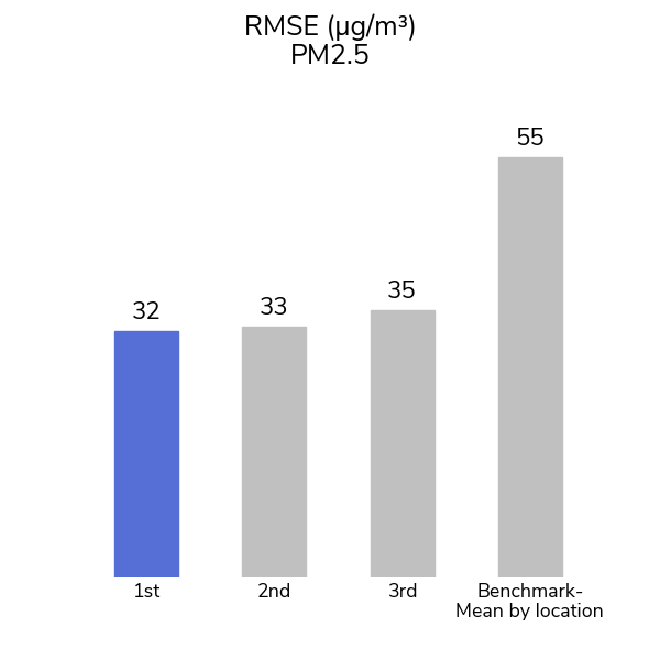
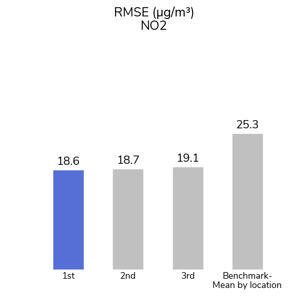
A second, simpler, benchmark was also used to contextualize the gains made by our winners on this problem: simply assigning the mean PM2.5 or NO2 level for each city within the training set as the prediction for cells in that city in the test set. This benchmark captures the variation between cities, but not the variation within a single city. Even so, this method achieved a leaderboard R-squared of 0.43 on the PM2.5 track and 0.03 on the NO2 track. To do better, competitors' models would have to learn the distinct patterns for each location.
The top models did indeed make significant gains, which is notable considering the sparsity of the satellite data and the vastly different distributions of pollutants in each location. The winners braved the world of possible datasets and in most cases integrated weather and elevation data as well to train their winning models.
|
|
|
|
Although the competitors used slightly different methods and datasets, there were a few common approaches between them:
-
Tree-based models: All six competitors made use of tree-based models. LightGBM was particularly popular among winners, citing that LGBM models are particularly suited to time series data with sparse inputs.
-
Imputation: Addressing missing data was a key part of winners' data preprocessing pipelines, given the gaps in satellite coverage. However, winners didn't agree on the best solution, with each performing imputation slightly differently.
-
Location-specific vs. overall training: Most winners chose to train separate location-specific models and ensemble them, while other trained on the entire dataset at once.
To learn more about each of the winning approaches, read on! The code for each winning submission is also available in our open-source competition winners repository
Meet the winners
| Place | PM2.5 Track | NO2 Track |
| 1st Place | Vishwas Chepuri | A. David Lander |
| 2nd Place | Raphael Kiminya | Raphael Kiminya |
| 3rd Place | Kudaibergen Abutalip | Sukanta Basu |
Vishwas Chepuri

Place: 1st Place, Particulate Matter Track
Prize: $12,000
Hometown: Nalgonda, Telangana, India
Username: vstark21
Background
I am a student pursuing an undergraduate degree in Electrical Engineering at the Indian Institute of Technology, BHU, Varanasi, India. My interests lie in Data Science and Machine Learning.
What motivated you to compete in this challenge?
For the past few months, I have been participating in competitions hosted on DrivenData. The last competition I participated in was related to cloud segmentation; this is when I developed an interest in working with remote sensing data. And these types of competitions are trying to solve certain problems around our environment and nature. So, contributing to this noble cause is one of the motivations.
Summary of approach
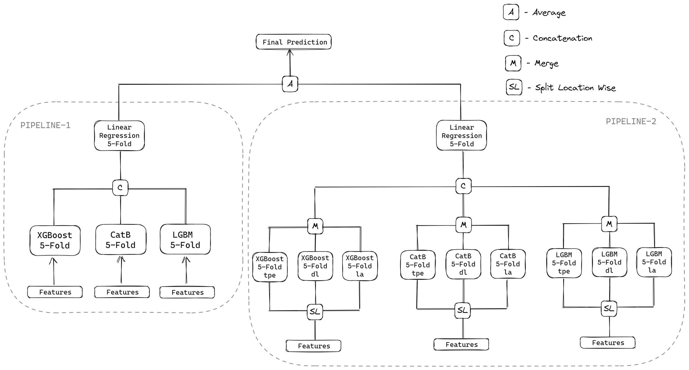
Firstly, raw data is processed, and then we impute the data using grid wise mean imputation method. After that, we generate temporal difference features and load metadata, and then train two pipelines. Check out the summary in the README.md and see the graphic below for more details on preprocessing and model architecture:
A. David Lander

Place: 1st Place, Trace Gas Track
Prize: $12,000
Location: United States
Username: _NQ_
Background
Winner, M5 Uncertainty Forecasting Competition First Place, Kaggle Coronavirus Forecasting Series Overall Winner of the U.S. Department of Justice Recidivism Forecasting Challenge
What motivated you to compete in this challenge?
I have a very strong background in time-series forecasting, and was looking to add geospatial forecasting experience.
Summary of approach
This is a classic time series forecasting situation, with only ~200 independent data points. The core of the challenge is ensuring robust cross-validation, very high regualization, and model averaging.
This includes purged KFold cross-validation with a ~30 day gap, fold and parameter rotation across each training iteration, and some clever parameter tuning. LightGBM is the gold standard for these situations, along with parameters selected intra-fold across every regularization option.
The most notable parameter was linear_tree, which fits a linear regression inside each leaf of the tree. I've never seen this used, but it worked very well for this competition given the strong (~0.4 - 0.6 in many cases) feature correlations with the target and limited set of data points.
Models were trained independently for all locations, and features were extracted using concentric circles around each grid point (0.05, 0.1, ... 5 degree radius).
A final ensemble with a neural network added an additional 0.5% to the model's performance.
Full details are in the public source code and a broader discussion is available in a forthcoming IJF article, Forecasting with Gradient-Boosted Trees: Augmentation, Tuning and Cross-Validation Strategies.
Raphael Kiminya

Place: 2nd Place, Particulate Matter and Trace Gas Tracks
Prize: $16,000
Hometown: Meru, Kenya
Username: karelds
Background
In my other life, I worked various roles as part of a data analytics team - as a systems admin, DBA, data warehouse architect and reports developer. I now work as a freelance data scientist. Over the past 2 years I’ve been studying machine learning through data competitions, solving all sorts of fascinating challenges.
What motivated you to compete in this challenge?
Satellites can "see" the air that we breathe? It’s ingenious. And I love a good challenge. Whenever I come across such a challenge, I’m reminded of the capacity of machine learning to alleviate the broader issues facing our society today. We can build solutions that affect millions of people, hopefully change their lives for the better.
Summary of approach
My approach was almost entirely data-centric. Initially I experimented with the original competition dataset and a variety of models. I quickly hit a plateau where local CV and LB scores didn’t improve.
I shifted my focus to the external datasets, and settled for a simple gradient boosting model to speed up my experiments. I used the MAIAC satellite data and GFS forecasts for the PM2.5 model. For the NO2 model, I used OMI and TROPOMI satellite data, GFS forecasts and GEOS-CF NO2 hindcasts.
Choice of GFS variables was based on relevant literature and availability of data throughout the training and testing period i.e. Jan 2017 to Aug 2021. Generally, I selected parameters affecting or similar to air humidity, soil temperature, soil humidity, air temperature, wind velocity, wind direction and rainfall/precipitation.
GFS forecasts from upto 3 days preceding the date of interest seemed to improve the predictions, so I created multiple datasets with different lookback periods. I also realized that separate models for each location performed better than a single model. Since the test set includes dataset from the past, I decided to use a k-fold (without shuffle) cross validation strategy instead of time-based splits. The final solution is an average ensemble of 45 models (3 datasets x 5 folds x 3 locations) and 30 models (2 datasets x 5 folds x 3 locations) for the NO2 model.
Kudaibergen Abutalip

Place: 3rd Place, Particulate Matter Track
Prize: $5,000
Hometown: Nur-Sultan, Kazakhstan
Username: Katalip
Background
My name is Kudaibergen Abutalip. Currently, I am a Master’s student in Computer Vision at the Mohamed bin Zayed University of Artificial Intelligence and residing in Abu-Dhabi, UAE. Originally, I am from Kazakhstan.
What motivated you to compete in this challenge?
In addition to the scale of the problem being tackled and its importance, introducing myself to a new domain and getting much more familiar with new concepts seemed exciting for me. Additionally, I was interested in working with geospatial data.
Summary of approach
The solution focuses on fusing approved Aerosol Optical Depth (AOD) data (MAIAC) and meteorological data (GFS). Several research papers have indicated the importance of complementing AOD data with such features [1, 2, 3]. The final model was an ensemble of tuned Random Forest Regressor and generalized Gradient Boosting Regressor from the sklearn library.
Data preprocessing approach:
AOD data is in HDF format and appropriate preprocessing steps outlined by organizers were followed: layer extraction, adding offset and scaling, constructing the grid in WGS84(EPSG:4326) coordinate system. As the data was in a raster format, mean, 95th percentile, min, max, standard deviation, variance of AOD values were extracted. The main problem with AOD data were missing values. Several approaches for time series imputation were tested, among which linear interpolation performed the best. Data was interpolated for each grid id separately while ensuring proper placement of data points (sorting by date).
GFS data variables were selected based on some investigation. For example, authors of one research paper about recent advances in PM2.5 forecasting and measurement indicate that meteorological factors might considerably affect PM2.5 concentration levels, and summarize correlation levels for rainfall, precipitation, wind speed, humidity, wind direction, atmospheric stability, relative humidity, daily average temperature, minimum temperature, maximum temperature. GFS data is distributed in grib2 format at 0.25° and was aggregated with respect to the product specifications. Grid coordinates at a finer resolution of each grid in three locations were rounded to the nearest GFS grid to join with AOD values.
Feature engineering steps that made into the final pipeline involved inclusion of year, month, and day derived features from the datetime column, wind magnitude from u and v directions of wind, mean encoding, label encoding, and addition of geospatial coordinates from grid metadata.
Modeling approach:
The final model was an ensemble of tuned Random Forest Regressor and generalized Gradient Boosting Regressor from sklearn library. The former model was tuned using 'Optuna' hyperparameter tuning framework (example in modelling_optuna.ipynb), while default hyperprameters without fixing the random seed for the latter were used. Some experimentation showed such an approach more effective for increasing overall generalization perfomance of the pipeline.
Sukanta Basu

Place: 3rd Place, Trace Gas Track
Prize: $5,000
Hometown: Delft, The Netherlands
Username: sukantabasu
Background
I am an associate professor at the Delft University of Technology, the Netherlands. My current research interests include turbulence modeling, numerical weather prediction, wind energy, atmospheric optics, and machine learning. Over the past fifteen years, my research has been funded by the US National Science Foundation (including an NSF-CAREER award), the US Department of Defense, the US Department of Energy, EU Horizon 2020 program, Carbon Trust (UK), TKI Wind op Zee (Netherlands), and other organizations. My research has been disseminated through more than 60 peer-reviewed journal publications.
What motivated you to compete in this challenge?
Over the past 2-3 years, I have been dabbling with state-of-the-art machine learning techniques and tools. This airathon was quite attractive as I was more-or-less familiar with the scientific content. I wanted to find out how my AIML skills matched up with top competitors.
Summary of approach
I used remote-sensing data from the Ozone Monitoring Instrument (OMI) and numerical weather prediction data from the Global Forecast System (GFS). For regression analysis, the LightGBM model is used in conjunction with an ensemble approach.
Thanks to all the participants and to our winners! Special thanks to the NASA MAIA and NASA TEMPO teams for enabling this important and interesting challenge!
Banner image courtesy of flickr user Clinton Steeds


