Overhead Geopose Challenge - Benchmark¶

Overhead satellite imagery provides critical time-sensitive information for use areas like disaster response, navigation, and security. Most current methods for using aerial imagery assume images are taken from directly overhead, or “near-nadir”. However, the first images available are often taken from an angle, or are “oblique”. Effects from these camera orientations complicate useful tasks like change detection, vision-aided navigation, and map alignment.

In the Overhead Geopose Challenge, your goal is to make satellite imagery taken from an angle more useful for time-sensitive applications like disaster and emergency response.

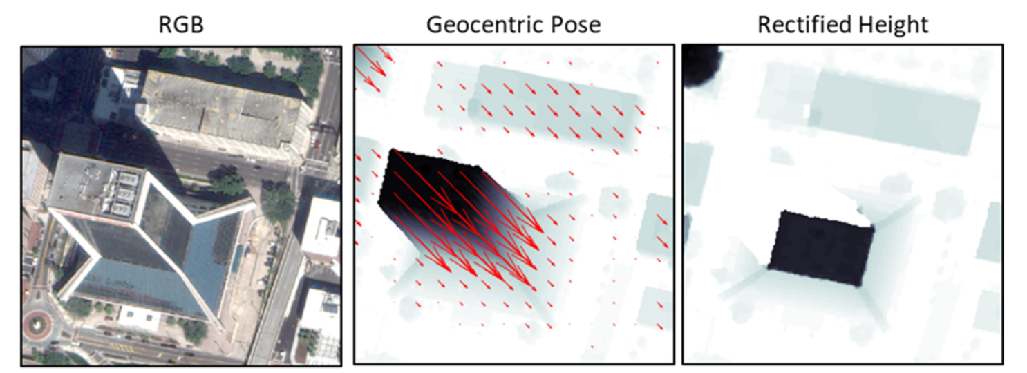
The features for this challenge are a series of RGB satellite images from four cities - Jacksonville, FL; Omaha, NE; Atlanta, GA; and San Fernando, ARG. Images from Jacksonville, Omaha, and San Fernando are cropped from publicly available WorldView (WV) 2 and WV-3 satellite data, provided courtesy of DigitalGlobe. Images from Atlanta were derived from the public SpaceNet dataset (see disclaimer). In this notebook, we go through the process of fitting a model that transforms each of these RGB images to its "geocentric pose". Geocentric pose is an object’s height above the ground and its orientation with respect to gravity. Calculating geocentric pose helps with detecting and classifying objects and determining object boundaries.

In this notebook, we'll cover:

• Getting set up
• Exploring the data
• Explaining the benchmark model
• Executing the benchmark model
• Generating a submission in the correct format

Let's get posing!

Disclaimer: Commercial satellite imagery is provided courtesy of DigitalGlobe. Atlanta images were derived from the public SpaceNet Dataset by SpaceNet Partners, licensed under a Creative Commons Attribution-ShareAlike 4.0 International License.

Getting Set Up¶

First, we'll import the basic tools we'll need to load our data and do some exploration.

If you have trouble installing packages, we recommend executing (in the command line):

conda install gdal cython opencv gdal tqdm scikit-image pytorch torchvision cudatoolkit -c pytorch
pip install segmentation-models-pytorch

And installing the remaining packages with pip install [package_name].

Now we can read in our data. You can find everything you need on the data download page.

What data do we have?¶

To get started, make sure to check out the data section of the problem description. The data set for this challenge includes satellite imagery from four cities: Jacksonville, Omaha, Atlanta, and San Fernando.

We're provided three datasets: metadata.csv, geopose_train.csv, geopose_test.csv

And four folders: train, test_rgbs, submission_format, train_nano

Metadata¶

Let's look at the metadata.

There are 6,948 images in the data. Our metadata has the following columns:

• id: a randomly generated unique ID to reference each record
• city: abbreviation for the geographic location
• gsd: ground sample distance (GSD) in meters per pixel. GSD is the average pixel size in meters.

Geopose data¶

We have geopose_test.csv and geopose_train.csv. Let's look at geopose_test.csv first.

There are 1,025 test records. Our test Geopose data has two columns:

• id: a randomly generated unique ID to reference each record
• rgb: name of the RGB image file, which is found in the test_rgbs folder

Based on the filepaths, we can see that RGB images have suffix .j2k. This means they are JPEG 2000 files. JPEG 2000 files offer compression similar to JPEG files, but are higher quality.

Now let's look at geopose_train.csv

There are 5,923 training images. Our train geopose data has columns for:

• id: a randomly generated unique ID to reference each record
• agl: name of the above ground level (AGL) height image file
• json: name of the JSON file with vector flow information (scale and angle)
• rgb: name of the RGB image file

The agl, json, and rgb files listed are all in the train folder. agl and json are part of what we are going to try to predict. They are provided for the training data, but not the test data.

AGL images have suffix .tif, meaning they are TIF images. TIFs are a high-quality graphics format. Since each pixel in our AGL image is only one value (height, cm), a lower-quality storage option would limit us to fairly low precision.

TAR files¶

The rest of the data is provided in tar.gz archives, or TARs.

• train: all training data files, including RGB images, AGL images, and JSONs with vector flow information
• test_rgbs: RGB images for the test data
• submission_format: An example submission that demonstrates correct submission format. All values are placeholder values
• train_nano: A small subset of 100 training records (RGB image, AGL image, and JSON vector flow for each). The nano set is provided for participants to more easily experiment with the data processing and modeling pipelines before running them on the full dataset.

For each TAR, let's extract all of the files to a regular directory using the tarfile library. Note that extraction takes a few moments.

Examine the training data¶

The train folder contains three types of files for each image:

• RGB image: JPEG 2000 file
• AGL height image: TIF file
• Vector flow information (scale and angle): JSON file

To more easily look through vector flow information, let's pull all of those JSONs into one dataframe first.

Now that we can see vector flow info more easily, let's look into a few records from the train folder. We can use the file names in geopose_train.csv.

For exploring images, we use the Image module from the Pillow package (version 8.2.0). Pillow is useful because it is easily able to work with TIF files and JPEG 2000 files, both of which we have in our data.

The RGB image is what we are given for the test set, and provides the features for the model. What we are trying to predict - our labels - is the AGL image with heights per pixel, the vector flow scale, and the vector flow angle. Together, these give us geocentric pose.

That was a very straightforward example - let’s look at another record that’s less clear.

Well that AGL image is odd! Checking the problem description again, we see that 65535 is used as a placeholder for nan values. The missing values in AGL arrays represent locations where the LiDAR that was used to assess true height did not get any data. You don't have to worry about height predictions for these pixels - pixels that are missing in the ground truth AGLs will be excluded from performance evaluation.

Let's get a more useful visual of that AGL. First, what's the max height that's actually recorded in the image?

It looks like the max height in the image is 2,949 cm (96 ft high). Now we can visualize again, and use the vmax argument:

Much better! We can see the image, and we can see where there are missing values.

What are the ranges for vector flow scale and angle?¶

To answer this question, let's first look at how many images there are for each city across both the train set and the test set. We know that there are four cities in the dataset. Based on the metric section of the problem description, our score will be calculated independently for each city, and then those four scores will be averaged to get our final performance.

• ARG: San Fernando, Argentina
• ATL: Atlanta, Georgia
• JAX: Jacksonville, Florida
• OMA: Omaha, Nebraska

San Fernando has much more data than the other three cities in both the train and test sets.

Let's check the range of vector flow scale (vflow_scale), and see whether it varies by city.

What did we learn?

• vflow_scale ranges from 0.0021 to 0.0153, and most of the images have a scale between 0.008 and 0.0125.
• This means that for most images, the average pixel size is between 0.008 pixels/cm and 0.0125 pixels/cm.
• Atlanta appears to be an exception and has lower scale values than other cities.

Per the data labels section of the problem description, scale is the pixels/cm conversion factor between vector field magnitudes in the 2D plane of the image and object height in the real world:

The geocentric pose vectors are all divided by numbers less than 0.0153 to get real-world height in cm. As expected, this means all of the images were taken from fairly far away and need significant magnification to match real-world height.

Now let's check vector flow angle (vflow_angle)

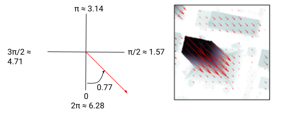
vflow_angle ranges from 0.0049 to 6.282. This matches our expectation - since angle is in radians, it can only have a value between 0 and 2$\pi$ = 6.283.

Atlanta has a much smaller range of vector flow scale and angle than any of the other three cities. Atlanta also has fewer images than the other cities, so overall there is a smaller range of satellite paths and possible camera angle in the data. By contrast, vector flow angle for San Fernando covers the full range of possibilities, indicating that there are many satellite paths and possible camera angles in the data.

What is the height range?¶

What heights are captured in the images and how does it vary by city? To get height, we can open individual AGL images and examine the image array.

Based on this sample of 250 images from each city, low pixel height values are fairly common - this is particularly true for Jacksonville and Omaha. In both of those cities at least 25% of pixels have a height of 0 cm. In Omaha half of pixels have a height less than 1 cm (0.4 inches), and Jacksonville is not much taller. That's pretty short! The vast majority of what is captured in the satellite images is relatively close to ground level.

Atlanta is the tallest city, but the majority of pixels are still not large enough to represent tall buildings. 50% of the pixels in Atlanta have a height less than 377 cm (12 ft) and 75% have a height less than 1,313 cm (43 ft).

This means very tall objects are pretty rare in the data, with Atlanta being somewhat of an exception.

Enough playing around. It's model time!

About the benchmark model¶

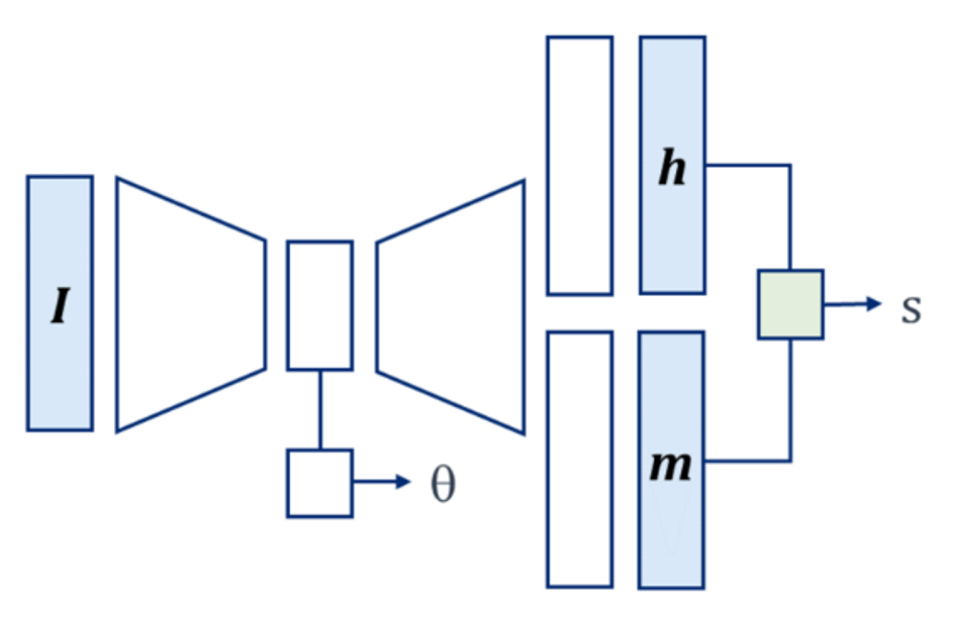
The benchmark code is a neural network built using the PyTorch library, created by the Johns Hopkins University Applied Physics Laboratory (JHU/APL). They parameterize the model in a multi-task deep network with a ResNet-34 encoder and U-Net decoder. The model estimates geocentric pose for image $I$ with:

The model uses the Adam optimizer with a learning rate of $1^{-4}$, which JHU/APL found to improve convergence over the default $1^{-3}$. We will train for 200 epochs.

The benchmark code relies on a number of different functions, specified in a handful of scripts. We will not go over every step of the model fitting process since it requires so many lines of code. Instead, we have shared the full benchmark code in a GitHub repository, and will review some key points here. Participants can clone the repo to access and run the full benchmark code. Our overview here is drawn from the thoughtful example write-up of the benchmark solution by JHU/APL.

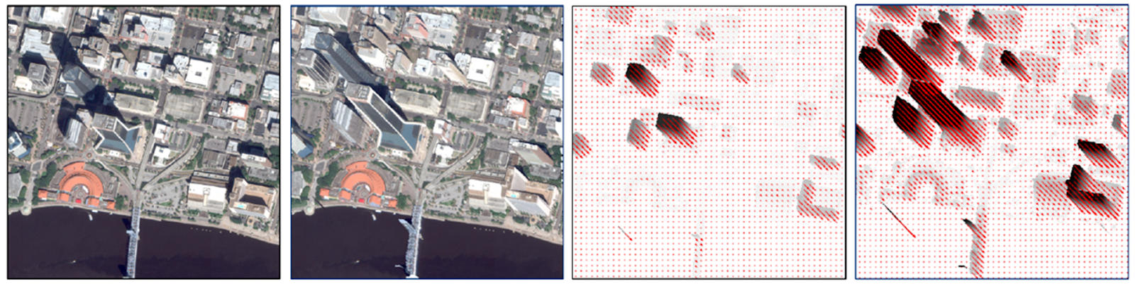
Taking advantage of affine projection

The benchmark regression model is designed to exploit the known affine relationship between object heights and their corresponding vector field magnitudes, which map surface-level features to ground level in an image. An affine transformation is a method of mapping variables in an image (ie. pixel values) to new variables by applying a linear combination of translation, rotation, and scaling. Affine transformation preserves the property of parallelism.

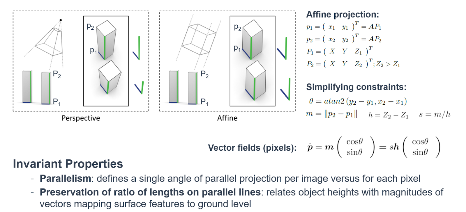
$\theta$ and $s$ are defined by the known relationship between vector field magnitudes $m$ (pixels) and objects heights $h$ (cm) from an affine camera, $s = m/h$.

Loss

The total loss $L$ that we'll minimize during training is a weighted sum of mean squared error (MSE) losses for all terms: $$ L=f_\theta L_\theta +f_s L_s + f_h L_h + f_m L_m $$

We set weighting factors $f_\theta=10$, $f_s=10$, $f_h=1$, and $f_m=2$ to normalize value ranges: $$ L=10 L_\theta + 10L_s + L_h + 2L_m $$

Note that for the loss equation above, scale is in pixels/meter and height is in meters.

For height and magnitude, MSE is calculated as the mean of MSE values for each labeled image in a batch to both reduce sensitivity to unlabeled pixels and allow for training images without height labels to directly supervise height and magnitude. In the latter case, height and magnitude MSE losses are zero and only the scale loss is back-propagated through those layers.

Augmentation to address bias

The distributions for angle of parallel projection $\theta$, scale factor $s$ relating height and magnitude, and object height $h$ are all heavily biased. Angle and scale are biased by the limited viewing geometries from satellite orbits, and very tall objects are rare. We'll encourage generalization and address bias with image remap augmentations $w_\theta$, $w_s$, and $w_h$. The function $w_\theta$ generates a new angle based on the original angle $\theta$ and some probability of an image's angle being augmented. Similarly, $w_s$ is a function of scale and probability, and $w_h$ is function of height and probability.

Image augmentation for rotation ($w_\theta$) and scale ($w_s$) are commonly applied to regularize training in deep networks, and depend only on image coordinates. This height augmentation ($w_h$) synthetically increases building heights. $w_h$ more specifically addresses the model's ability to accurately predict height for very tall objects, even though they are rare in the training data set.

The following high-level code from utilities/augmentation_vflow.py applies height and rotation augmentation:

def augment_vflow(image, mag, xdir, ydir, angle, scale, agl=None, rotate_prob=0.3, flip_prob=0.3, scale_prob=0.3, agl_prob=0.3):
    # increase heights
    if np.isnan(mag).any() or np.isnan(agl).any():
        agl_prob = 0
    if random.uniform(0, 1) < agl_prob:
        max_agl = np.nanmax(agl)
        max_building_agl = 200.0
        max_factor = 2.0
        max_scale_agl = min(max_factor, (max_building_agl / max_agl))
        scale_height = random.uniform(1.0, max(1.0, max_scale_agl))
        image, mag, agl = warp_agl(image, mag, angle, agl, scale_height, max_factor)

    # rotate
    if random.uniform(0,1) < rotate_prob:
        rotate_angle = random.randint(0,359)
        xdir,ydir = rotate_xydir(xdir, ydir, rotate_angle)
        image,mag,agl = rotate_image(image, mag, agl, rotate_angle)

     ...

warp_angle is also defined in utilities/augmentation_vflow.py.

Note that shadows are not adjusted by this simple but effective augmentation. Relying too much on shadows in model training can be risky because they are only sometimes observed. Maybe YOU could be the one to figure a better way to take advantage of hints from the shadows!

Recap

We're going to use a deep neural network to predict geocentric pose. A couple of our key objectives are:

• Take advantage of what we know about affine projection to define the relationship between objects heights and vector magnitudes, $\textrm{scale} = \frac{\textrm{object height}}{\textrm{vector magnitude}}$
• Use image augmentation to address some of the bias in the data. In particular, by synthetically increasing building heights to correct for how rare tall objects are in the data.
• Define loss - what we are going to minimize - as a weighted sum of MSE losses for vector flow angle ($L_\theta$), vector flow scale ($L_s$), object height ($L_h$), and vector flow magnitude ($L_m$)
• Tools: PyTorch library, ResNet-34 encoder, and U-Net decoder

Executing the benchmark model¶

1. Clone the repo¶

In the command line, enter git clone https://github.com/pubgeo/monocular-geocentric-pose.git

Let's take a look at the files in the benchmark repo:

benchmark
├── utilities
│   ├── augmentation_vflow.py
│   ├── cythonize_invert_flow.py
│   ├── downsample_images.py
│   ├── evaluate.py
│   ├── invert_flow.pyx
│   ├── misc_utils.py
│   ├── ml_utils.py
│   └── unet_flow.py
├── README.md
└── main.py

• main.py: Defines the command line function that runs training and testing. Once arguments are passed to the command line, main.py calls functions in other scripts based on those arguments.

In utilities:

• augmentation_vflow.py: implements affine transformation and augmentation - $w_\theta$, $w_s$, and $w_h$ as discussed above
• downsample_images.py: down-samples images from a directory and creates a directory at half resolution. This reduces memory requirements and enables model training to use larger batch sizes. When the benchmark was trained on half-resolution data, there was no reduction in prediction accuracy
• evaluate.py: gets the performance metrics (R-squared) for each city and returns the average across cities. This code is what will be used to judge participant submissions. This script can also be called to write rectified height images.
• misc_utils.py: miscellaneous functions that are used across scripts - eg. saving images, loading images, and calculating Root Mean Squared Error (RMSE).
• ml_utils.py: implements training and testing using PyTorch
• unit_vflow.py: defines the Unet model class used in ml_utils.py, including encoders and key methods for training like forward and predict
• invert_flow.pyx: code for inverting the flow written in python-type syntax, but able to be parsed by Cython.
• cythonize_invert_flow.py: compiles the invert_flow function

Part of the height augmentation is inverting the vector flow, which is done through invert_flow.pyx and cythonize_invert_flow.py. The code for inverting flow in invert_flow.pyx loops over every row and column of each image. This would run VERY slowly in python, so is implemented using Cython to improve speed. Cython is a compiler that allows you to write code in python that will be compiled and executed in C, but is still able to communicate with the rest of the code written in python. Running code in C rather than python significantly increases computational efficiency.

2. Set up environment¶

If you did not run the conda install command from Getting set up, you should now run:

conda install gdal cython opencv gdal tqdm scikit-image pytorch torchvision cudatoolkit -c pytorch
pip install segmentation-models-pytorch

In addition to the dependencies listed in setup, here we will build the invert_flow Cython function by executing (in the command line):

cd utilities
python cythonize_invert_flow.py build_ext --inplace

3. Down-sample training data¶

The benchmark is trained with images down-sampled by a factor of two (i.e. at half resolution). It is tested with full-resolution images. We found that training on half-resolution images did not decrease prediction accuracy, but did save time.

Tip: You can execute shell commands in a Jupyter notebook by adding ! before the code, eg. !cd utilities

4. Train¶

We will train for 200 epochs. Command line arguments are explained in main.py.

Be aware that training the model can take a long time, up to multiple days. With 200 epochs, it took our benchmark a little less than three days to run using a Tesla T4 GPU (about 20 minutes per epoch). Before training on the full data set with your final hyperparameters, we recommend testing your pipeline by training with a small number of epochs and/or on a small "nanoset" of the data, like the one provided on the data download page.

To make sure we don't lose any work if we are disconnected from our remote ssh session, we used tmux to launch our Jupyter notebook and run the model training. In our notebook, we will set up the training cell to print to a .txt file rather than in the notebook.

To see the model's progress:

!tail -2 {str(DATA_PATH / "training.txt")}

Epoch: 199
train: 100%|█| 1185/1185 [19:24<00:00,  1.02it/s]

The benchmark code saves Pytorch model checkpoints throughout training in the directory specified by the --checkpoint-dir command line argument. Even though model training has the potential to get interrupted, you should always be able to pick back up where you left off without having to restart training from scratch.

The benchmark does not set aside part of the training data for validation. We recommend that you add a validation step.

Generating a Submission¶

Now that our model is trained, we are finally ready to perform inference and make a submission. You'll only want to perform inference on the test set once you determine your top performing model, to avoid inadvertently overfitting.

First, let's look at the submission format¶

Submissions have to match the submission format from the problem description. In the data provided, there is a submission_format folder that demonstrates the correct submission format with placeholder values. You can check your submission against the format folder to make sure it is in the correct format and has the right files.

For each image in the test_rgbs folder, the submission format contains two files:

1. A 2048 x 2048 .tif file with height predictions. The name of the AGL file should be [city_abbreviation]_[image_id]_AGL.tif. AGLs should show height in centimeters and have data type uint16.
2. A JSON file with vector flow information. The name of the JSON file should be [city_abbreviation]_[image_id]_VFLOW.json. Scale is in pixels/cm. Angle is in radians, starting at 0 from the negative y axis and increasing counterclockwise.

For more details and an explanation of vector flow scale and angle, see the section on data labels in the problem description.

Run inference on the test data¶

Since the model was trained with 2x down-sampled images, we set downsample=2. This down-samples the test images before making predictions, so that they better match the way the model was trained. Predictions are then up-sampled before writing output files.

The dataset specified consists of test set RGBs, downloaded from the competition data page.

submission now has everything we need to make a submission!

Check against the submission format¶

To make sure we have all of the right files, we can check that every file in the submission format appears in our predictions folder.

Success, we have all of the right files! However, our predictions folder takes up a lot of space - roughly 8.6 GB.

Compress TIF files¶

Our predictions were generated as float values in meters. To make the size of participant submissions manageable, we'll convert pixel values to centimeters and store as data type uint16. Submissions are expected to be in centimeters and pixel heights in any other unit will not be scored correctly. Submission AGL images should also be saved using a lossless TIFF compression. In the benchmark, we compress each AGL TIFF by passing tiff_adobe_deflate as the compression argument to the Image.save() function from the Pillow library.

In our command to run inference above, we set --convert-predictions-to-cm-and-compress=False in order to walk through these steps explicitly. Setting that argument to True accomplishes the same thing by calling this function.

Our new, shiny, compressed submission folder only takes up roughly 1.7 GB! Much better.

Save into a TAR archive¶

The required submission format for the platform is a TAR file (.tar.gz) - other formats will be rejected and not scored. We use the tarfile library to create a TAR and then add all of our submission files.

Your final submission .tar.gz should be around 1.6 GB. Submissions that are very large will be rejected by the platform.

You're ready to submit!¶

Head over to the competition submissions page and click "Make new submission". Upload submission_compressed.tar.gz.

Congrats! We got a final R-squared of 0.7996. Not bad, but definitely room for improvement. Some of the main instances when the benchmark does not perform well are buildings that:

• Have an unusual appearance or shape
• Are observed from very oblique viewpoints, which can make the building appear unusual or oddly shaped
• Have no hints observed in the image from shadows

In particular, any taller buildings that fall into these categories are difficult to predict.

A couple of ideas to explore for improving the benchmark:

• Architectural improvements to the workhorse U-Net decode with ResNet34 backbone
• Ensemble methods
• Additional creative augmentations to improve image generalization
• Optimizations to improve training efficiency, since the images are so large
• Innovative loss functions. For example, noisy height predictions can be inconsistent with input image gradients along roof boundaries, and we did not experiment with additional priors in the loss function. It might also be interesting to experiment with surface normal loss, as that has been shown to improve accuracy in depth prediction tasks.

This competition has a bonus model write-up track. The example writeup of the benchmark solution is a good place to look for more details on suggested improvements (question 7), as well as general model explanation.

Check out the Overhead Geopose Competition challenge homepage to get started. We can't wait to see what you build!

Approved for public release, 21-553.