Forecasting Energy Consumption
Background
Building energy forecasting has gained momentum with the increase of building energy efficiency research and solutions. Indeed, forecasting the global energy consumption of a building can play a pivotal role in the operations of the building. It provides an initial check for facility managers and building automation systems to mark any discrepancy between expected and actual energy use. Accurate energy consumption forecasts are also used by facility managers, utility companies and building commissioning projects to implement energy-saving policies and optimize the operations of chillers, boilers and energy storage systems.
Planning and forecasting the use of electrical energy is the backbone of effective operations. Energy demand forecasting is used within multiple Schneider Electric offers, and different methods require more or less data. Schneider Electric is interested in more precise and robust forecasting methods that do well with little data.
** In this competition data scientists all over the world built algorithms to forecast building consumption reliably. **
The best algorithms were generally ensembles of models with modelers that thought very, very carefully about how to avoid using future data in their time series models. Using weather, holidays, synthetic features, and LightGBM, these participants created the best predictions!

Meet the winners below and hear how they applied machine learning to the important challenge of forecasting building energy use!
Meet the winners
Andrey Filimonov

|
Place: 1st
Prize: €12,000
Hometown: Moscow, Russia
Username: slonoslon
Background:
Most of my career was in software development: from writing simple tools to building large-scale IT systems. Currently I split my working time between two jobs: teaching (I teach children robotics at Moscow school 654) and fintech (building machine learning models to predict future market prices).
Summary of approach:
First, I did a lot of preprocessing (history-based aggregate functions calculation) of original data to produce features for each point in train and test sets. Then, these features are used to train gradient boosting (LightGBM) model.
Check out Andrey’s full write-up and solution in the competition repo.
Jacques Peeters

Place: 2nd
Prize: €7,000
Hometown: Paris, France
Username: jacquespeeters
Background: Graduated in 2016 from Polytech Lille in Software Engineering and Statistics. Currently moving from a Data Scientist role in a consulting firm to a more machine learning oriented role in an online marketplace.
Summary of approach: I did not predict the value directly, but value / value_mean where value_mean is the mean value of the building during the Tn last available timestamp. With Tn the size of the timestamp forecast (the number of timestamps that we are calculating the metric over for this forecast n).
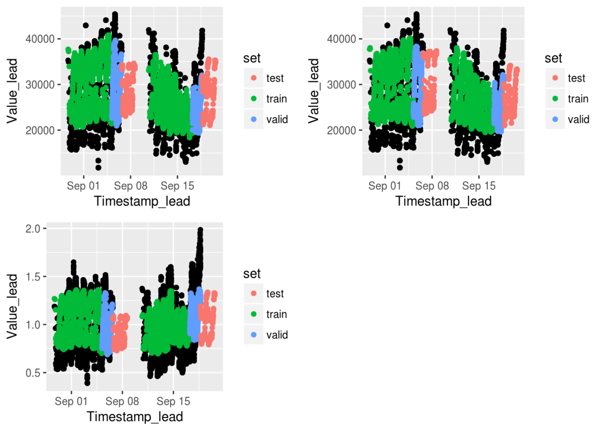
For each timestamp, match I find the closest: a. Last available values b. Last available values on (time) c. Last available values on (time, day of week) d. Last available values (time, close) (with the same business day (close/open))
Then, I compare weather to the above matching to the timestamp to be predicted. Each timestamp can be predicted from different t (with 0 < t <= Tn), therefore each timestamp generate up to Tn learning points. It generates more than one billions points which I couldn’t handle locally. Therefore I sampled around X millions rows (therefore my models are trained only on X% of the possible learning data) them given their weight in the metrics.
The final model is a simple average of 3 LightGbm models with different set of parameters (number of leaves). The mdoels have a time series specific training process: train and validate models with time split in order to avoid any leak (in my case determine the number of iterations), then re-train on full data before predicting
In the end, there is 6 models trained (3 set of parameters, once on train/valid, once on full data) on all 300 Building/SiteId. It takes around 2 hours to train.
Check out jacquespeeters's full write-up and solution in the competition repo.
Will Koehrsen

Place: 3rd
Prize: €4,000
Hometown: Cleveland, OH, USA
Username: willkoehrsen
Background:
I am a Master’s student in mechanical engineering with a research focus in applied data science at Case Western Reserve University. I have an undergraduate degree in mechanical engineering and am almost entirely self-taught (using Udacity, Coursera, and books) when it comes to data science. I work on a research project called Energy Diagnostic Investigator for Efficiency Savings (EDIFES) that uses large- scale data analytics to improve building energy efficiency. My long term goals are to graduate with my Masters next year (May 2019) and work full time as a data scientist in the clean technology sector, preferably for a start-up working to enable the transition to a renewable energy economy.
Summary of approach:
My approach treats the problem as a standard supervised regression task. Given a set of features – the time and weather information – we want to build a model that can predict the continuous target, energy consumption. The model is trained on the past historical energy consumption using the features and the target and then can be used to make predictions for future dates where only the features are known.
I first engineered the original training and testing data to extract as much information as possible. This involves first breaking out the timestamp into minutes, hours, weekday, day of the year, day of the month, month, and year. The time variables are then converted to cyclical features to preserve the proper relationships between times (such as hour 0 being closer to hour 23 than to hour 5). Then I joined the weather data to the building energy-use data because the temperature can significantly influence the energy consumption and including this information helps the model learn to predict energy use. I rounded the index of the weather data to the nearest fifteen minutes and then joined the weather data to the building energy-use data based on the timestamp. The final aspect of feature engineering was finding the days off for each building using the metadata. This is crucial because the energy use differs significantly between working and non-working days. The same engineering that was applied to the training data was applied to the testing data because the model needs to see the same features at test time as during training. I did not include the holidays in the data because I found the information was sparse.
The final machine learning model I built is an ensemble of two ensemble methods (a meta-ensemble I guess you could call it), the random forest and the extra trees algorithms. The final model is made up of six random forest regressors and six extra trees regressors, each of which uses a different number of decision trees (from 50 to 175 spaced by 25). (All of the algorithms are implemented using the Scikit- learn Python library). The final predictions are made by averaging the results of these 12 individual estimators. During training, I train the complete model on a single building at a time, which I found to work best rather than trying to make one model that can be trained on all buildings at once. I first select the engineered training and testing data for the ForecastID, making sure to use only past data for training. Then, I impute the missing temperature values in the training and testing data using median imputation. I impute the missing energy values only in the training data using median imputation (this is not done for the testing data because the energy value is what we want to predict). I convert the timestamp to a numeric value so the machine learning models can understand this feature, and make sure to drop the energy use value from the training data. The random forest and extra trees models do not require features to be scaled, but for other machine learning models, scaling the features between 0 and 1 is a best practice so this step is implemented before the models are trained.
For each building, I then train the 12 separate models on the training data and make predictions on the testing data. The final predictions are made by averaging the predictions from the 12 individual models. Once predictions have been made for all buildings, they are saved to the specified file.
Check out willkoehrsen’s full write-up and solution in the competition repo.
Thanks to all the participants and to our winners! Special thanks to Schneider Electric for a fascinating challenge!

