How to predict PM2.5 using MAIAC Aerosol Optical Depth data
Welcome to the getting started notebook for the particulate track of the NASA Airathon: Predict Air Quality challenge! The goal of this tutorial is to provide some helpful pointers and starter code to ingest, preprocess, explore, and work with one of the atmospheric data products derived with data from the Moderate Resolution Imaging Spectroradiometer (MODIS) instrument onboard the Terra and Aqua satellites. The specific scientific parameter covered by this tutorial is called Aerosol Optical Depth (AOD). AOD is derived from an algorithm called Multi-Angle Implementation of Atmospheric Correction (MAIAC) and is made available in Hierarchical Data Format (HDF). If MODIS, MAIAC, AOD, PM2.5, or HDF are new concepts to you, then read on!
Before getting started, check out the Airathon competition homepage to learn more about the goal of this important challenge. In this tutorial, we'll:
- Provide an overview of some key concepts
- Explore the competition metadata
- Demonstrate how to load data in HDF4
- Clean, align, and reproject MAIAC data
- Build a rudimentary model to predict particulate matter levels
Let's get started!
The Data
What is MAIAC?
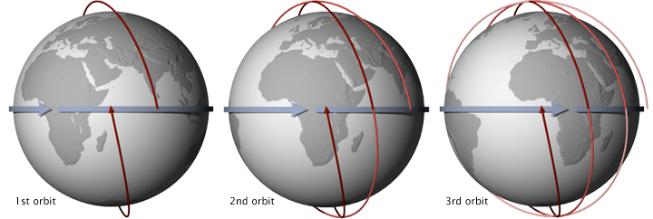
Terra and Aqua are NASA scientific research satellites that orbit the Earth to study Earth's various natural systems. Terra passes from north to south across the equator in the morning, while Aqua passes from south to north over the equator in the afternoon. Their orbits are sun-synchronous, meaning that they pass the equator at the same local solar time on every orbit.
MODIS is the name of two remote sensing instruments administered by NASA aboard the Terra and Aqua satellites. MODIS has provided Earth observation data in 36 spectral frequencies of light at 250 meters to 1 km resolution since the launch of Terra in 1999. Because of its extensive coverage, MODIS enables researchers to monitor activities spanning from active fires, smoke, and dust storms to changes in land use. Together, the two MODIS instruments are able to capture the entire Earth's surface every one to two days.
MAIAC is an algorithm that combines pixel- and image-based processing to improve the accuracy of the aerosol, cloud, and atmospheric data retrieved from MODIS. The algorithm translates MODIS Level 1B measurements to a fixed grid at 1 km resolution in order to observe the same grid cell over time. This correction allows us to work with polar-orbiting observations as if they were geostationary and makes it easier to characterize surface backgrounds and conduct time series analyses. MAIAC provides a suite of aerosol and land surface reflectance products in HDF4 format.
This exercise will focus on the MCD19A2 Version 6 gridded Level 2 product. Level 2 products represent geophysical variables derived from raw instrument and payload data (e.g., Level 1B).
What is AOD?
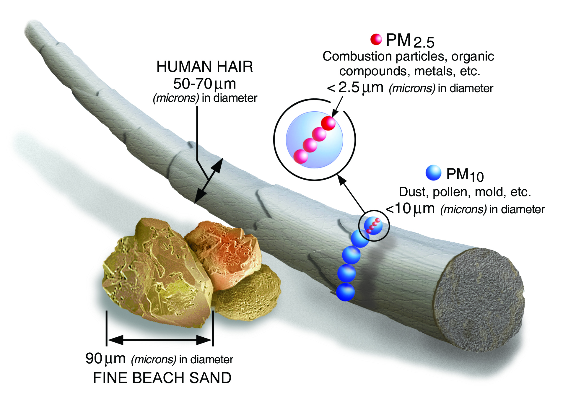
MCD19A2 reports Aerosol Optical Depth (AOD) collected daily at 1 km resolution. AOD, also called Aerosol Optical Thickness (AOT), is a unitless measure of aerosols distributed within a column of air from Earth's surface to the top of the atmosphere. AOD has been found to be helpful for estimating the presence of harmful air pollutants including PM2.5, or particulate matter that's less than 2.5 micrometers (µm) in diameter. AOD and PM2.5 are a critical air quality measures because particulates can penetrate deep into the lungs, increasing the risk of health complications like lower respiratory infections or heart disease.
While the MCD19A2 data product contains a variety of Science Dataset (SDS) layers, we will focus on blue band AOD at 0.47 µm. It's worth noting that MAIAC also uses this value and regional aerosol models to compute green band AOD at 0.55 µm. You are encouraged to explore and leverage all of the layers made available by this data product using the MAIAC Data User Guide.
Data loading
What's in our metadata?
First, let's organize our local repository using Cookiecutter Datascience and download the grid_metadata.csv, pm25_satellite_metadata.csv, submission_format.csv, and train_labels.csv files from the data download page to our data/raw folder.
$ tree data/
data/
├── external
├── interim
├── processed
└── raw
    ├── grid_metadata.csv
    ├── pm25_satellite_metadata.csv
    ├── submission_format.csv
    └── train_labels.csv

4 directories, 4 files
Next, let's import some handy tools for working with geospatial data and load the metadata to see what we have.
from pathlib import Path
import random
from typing import Dict, List, Union

from cloudpathlib import S3Path
import geopandas as gpd
import pandas as pd
import rasterio

DATA_PATH = Path.cwd().parent / "data"
RAW = DATA_PATH / "raw"
INTERIM = DATA_PATH / "interim"
pm_md = pd.read_csv(
    RAW / "pm25_satellite_metadata.csv",
    parse_dates=["time_start", "time_end"],
    index_col=0,
)

grid_md = pd.read_csv(RAW / "grid_metadata.csv", index_col=0)
Satellite metadata
Our particulate track satellite metadata file contains information about MAIAC and MISR data made available for model training and testing. Since we'll be focusing on preparing MAIAC training data, let's create and inspect a subset.
pm_md.columns
pm_md["split"].value_counts()
pm_md["product"].value_counts()
maiac_md = pm_md[(pm_md["product"] == "maiac") & (pm_md["split"] == "train")].copy()
maiac_md.shape
maiac_md.head(3)
As MODIS sweeps along an orbit, it collects data that is sectioned into pieces called granules. Each MAIAC granule contains 13 SDS layers and has a size of 1200 x 1200 pixels representing 1200 x 1200 km. Each granule is identified by a unique granule_id with the following naming convention: {time_end}_{product}_{location}_{number}.hdf, where time_end is formatted as YYYYMMDDHHmmss. When locations and times have more than one associated file, this is denoted by number. For additional information about each of these fields, check out the PM2.5 data download instructions.
We can see that there are 4,260 MAIAC files to use for training. Each file corresponds with one of the three competition locations: Los Angeles South Coast Air Basin, Delhi, or Taipei. Let's take a look at the distribution of granules by location.
maiac_md.location.value_counts()
Taipei has twice as many associated files as Los Angeles or Delhi. This is to be expected, because two separate orbit tracks bisect Taipei, i.e., one track covers half of Taipei and another covers the other half.
We can also take a look at the time distribution in our training data.
maiac_md.time_end.dt.year.value_counts()
maiac_md.time_end.dt.month.value_counts().sort_index()
We have a roughly balanced distribution of files across years (2018-2020) and months, with the fewest granules from the month of January.
(maiac_md.time_end - maiac_md.time_start).describe()
A single granule contains data that was captured within a time window spanning from 5 minutes to 14+ hours, with an average timeframe of around 1.5 hours.
Grid metadata
Next, let's take a look our grid cell metadata.
grid_md.head(3)
grid_md.shape
grid_md.location.value_counts()
Each grid cell is identified by a 5-character alphanumeric grid_id that uniquely identifies a 5 x 5 km grid cell and is associated with an observation in our train or test set. This file also contains important location and timezone (tz) information that can be used to localize dates, along with the polygonal coordinates of the grid cell.
We can see that there is metadata available for 54 grid cells.
How do I load a MAIAC HDF4 file?
Our MAIAC data is stored in a HDF4 file format. At its lowest level, Hierarchial Data Format (HDF) is a set of file formats (HDF4 and HDF5) designed to store and organize large amounts of scientific data. HDF4 is the older version of the format, but is still actively supported by a non-profit corporation called The HDF Group. This file format supports different data models, including multidimensional arrays, raster images, and tables. A single HDF file can hold a mix of related objects that can be accessed as a group or as individual objects.
In Python, we can read in HDF4 files using one of three libraries:
For this example, we'll be using PyHDF and code adapted from a script on the HDFEOS zoo. The SD module of the pyhdf package supports scientific datasets. Let's import this module along with some helpful tools to get started.
import os
import re

import numpy as np
import matplotlib as mpl
import matplotlib.pyplot as plt
from pyhdf.SD import SD, SDC, SDS
import pyproj

mpl.rcParams["figure.dpi"] = 100
The MAIAC metadata file contains the locations of each MAIAC HDF4 file on s3. We can use the S3Path class from the cloudpathlib package to generate a path to a sample data file from Los Angeles.
la_file = maiac_md[maiac_md.location == "la"].iloc[0]
la_file_path = S3Path(la_file.us_url)
la_file_path
To read this file, we can instantiate an SD object using a string representation of our path along with a file opening mode of SDC.READ. Note that calling fspath downloads the file locally to a temporary directory.
hdf = SD(la_file_path.fspath, SDC.READ)
hdf.info()
Path(la_file_path.fspath).unlink()
Our hdf object contains 13 datasets or bands and 8 attributes. We are most interested in the dataset related to blue band AOD at 0.47 µm (Optical_Depth_047).
We can list the 13 available datasets by calling the datasets method on hdf.
for dataset, metadata in hdf.datasets().items():
    dimensions, shape, _, _ = metadata
    print(f"{dataset}\n    Dimensions: {dimensions}\n    Shape: {shape}")
Dataset attributes
To load the Optical_Depth_047 dataset, we'll use the select method on our hdf object.
blue_band_AOD = hdf.select("Optical_Depth_047")
name, num_dim, shape, types, num_attr = blue_band_AOD.info()

print(
    f"""Dataset name: {name}
Number of dimensions: {num_dim}
Shape: {shape}
Data type: {types}
Number of attributes: {num_attr}"""
)
According to our metadata, the blue band AOD data contains 3 dimensions. The first dimension represents the number of orbit overpasses or timestamps contained in the file (four in Los Angeles), while the second and third dimensions represent the height and width of a single band, i.e., 1200 x 1200 pixels. There are more overpasses at the poles (up to 30) and fewer at the equator (1-2). At high latitudes, only the first 16 orbits with the largest coverage are selected for processing per day. A data type of 22 represents a signed 16-bit integer according to the SDC constants.
To access the raw data, simply call get on the AOD blue band dataset object.
blue_band_AOD.get()
In order to work with the data, we'll need to calibrate the raw values by applying a set of accompanying attributes, including the following:
- scale factor
- offset
- missing data value
- valid value range
Let's save these values for later.
calibration_dict = blue_band_AOD.attributes()
calibration_dict
HDF file attributes
We'll also need to save a few attributes from the file's metadata to align and reproject our data into a usable representation. More specifically, we'll need:
- upper left coordinate of the granule
- lower right coordinate of the granule
- projection
- projection parameters
All of this information can be parsed from an attribute on hdf called StructMetadata.0.
list(hdf.attributes().keys())
raw_attr = hdf.attributes()["StructMetadata.0"]
print(raw_attr)
As we saw above, Optical_Depth_47 is available at 1 km resolution, so we'll use the first group of metadata (i.e., GridName="grid1km") and convert the relevant fields into a dictionary.
# Construct grid metadata from text blob
group_1 = raw_attr.split("END_GROUP=GRID_1")[0]
hdf_metadata = dict([x.split("=") for x in group_1.split() if "=" in x])

# Parse expressions still wrapped in apostrophes
for key, val in hdf_metadata.items():
    try:
        hdf_metadata[key] = eval(val)
    except:
        pass

hdf_metadata
Now that our metadata is parsed, we can save the attributes we'll need to align and reproject our data.
# Note that coordinates are provided in meters
alignment_dict = {
    "upper_left": hdf_metadata["UpperLeftPointMtrs"],
    "lower_right": hdf_metadata["LowerRightMtrs"],
    "crs": hdf_metadata["Projection"],
    "crs_params": hdf_metadata["ProjParams"],
}
alignment_dict
Data processing
Now that we have our calibration_dict, alignment_dict, and raw data (blue_band_AOD), we have everything we need to calibrate and map AOD values to the competition grid cells.
How do I calibrate AOD data?
To calibrate our data, we'll loop through each orbit and apply a set of corrections based on the information contained in the calibration_dict:
- remove values that fall outside of the
valid_range(-100 to 5000) - remove missing data (indicated by a
_FillValueof -28672) - remove any
offset(none in this case) and multiply by thescale_factor(0.0001) - cast the data to a numpy masked array to handle missing entries
Note: Values outside of the valid range can't be used because they fall outside of the scope of the MODIS sensor, and the fill value donates low quality readings. This can happen for a number of reasons, including cloud cover or reflectance from snow or water. In the following code we'll consider both invalid and convert them to nans.
# Loop over orbits to apply the attributes
def calibrate_data(dataset: SDS, shape: List[int], calibration_dict: Dict):
    """Given a MAIAC dataset and calibration parameters, return a masked
    array of calibrated data.

    Args:
        dataset (SDS): dataset in SDS format (e.g. blue band AOD).
        shape (List[int]): dataset shape as a list of [orbits, height, width].
        calibration_dict (Dict): dictionary containing, at a minimum,
            `valid_range` (list or tuple), `_FillValue` (int or float),
            `add_offset` (float), and `scale_factor` (float).

    Returns:
        corrected_AOD (np.ma.MaskedArray): masked array of calibrated data
            with a fill value of nan.
    """
    corrected_AOD = np.ma.empty(shape, dtype=np.double)
    for orbit in range(shape[0]):
        data = dataset[orbit, :, :].astype(np.double)
        invalid_condition = (
            (data < calibration_dict["valid_range"][0])
            | (data > calibration_dict["valid_range"][1])
            | (data == calibration_dict["_FillValue"])
        )
        data[invalid_condition] = np.nan
        data = (data - calibration_dict["add_offset"]) * calibration_dict["scale_factor"]
        data = np.ma.masked_array(data, np.isnan(data))
        corrected_AOD[orbit, ::] = data
    corrected_AOD.fill_value = np.nan
    return corrected_AOD
corrected_AOD = calibrate_data(blue_band_AOD, shape, calibration_dict)
corrected_AOD
pd.DataFrame(corrected_AOD.ravel(), columns=["AOD"]).describe()
How do I align AOD data with coordinates?
Using our alignment_dict, we can now align each corrected AOD pixel with grid coordinates. From there, we will be able to determine which AOD readings overlap with our training grid cells.
We will follow four steps to map values in a 2-dimensional matrix to 3-dimensional "world" coordinates. This process is known as georeferencing:
- identify the original coordinate reference system (CRS) of the dataset
- define reference points on our grid
- perform any necessary reprojections of these points
- connect points to AOD values
We can choose to use one of two georeferencing approaches: vector- or raster-based. You may choose to use one or the other based on computational performance, memory usage, and/or library preferences.
Vector data is composed of discrete geometric locations, or vertices, that define the shape of a spatial object (e.g. points, lines, or polygons). Each feature can carry multiple attributes about a location. Geospatial vector data can be used with the convenient geopandas.GeoDataFrame class.
Raster data is stored as a grid of values that are rendered on a map as pixels, where each pixel value represents an area on the Earth's surface. Raster data is useful for representing continuous surfaces at high levels of detail and for performing efficient geometric computations. Rasters are commonly saved as GeoTIFFs, which contain geographic metadata.
Vector-based approach
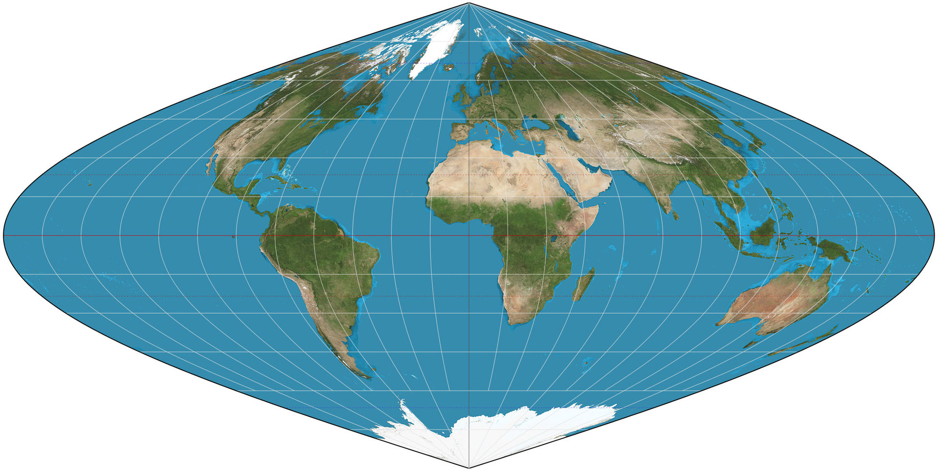
Step 1: A CRS defines the mathematical approach used to transform real locations on the Earth into a flattened map. The CRS of our data is the sinusoidal projection according to our alignment_dict (GCTP_SNSOID). As an equal-area map projection, the sinusoidal projection preserves area while distorting shapes.
Step 2: Next, using the coordinates of the granule's upper_left and lower_right coordinates, we'll create a rectangular mesh grid of 1200 x 1200 evenly spaced points in the same projection as these coordinates.
shape
alignment_dict
def create_meshgrid(alignment_dict: Dict, shape: List[int]):
    """Given an image shape, create a meshgrid of points
    between bounding coordinates.

    Args:
        alignment_dict (Dict): dictionary containing, at a minimum,
            `upper_left` (tuple), `lower_right` (tuple), `crs` (str),
            and `crs_params` (tuple).
        shape (List[int]): dataset shape as a list of
            [orbits, height, width].

    Returns:
        xv (np.array): x (longitude) coordinates.
        yv (np.array): y (latitude) coordinates.
    """
    # Determine grid bounds using two coordinates
    x0, y0 = alignment_dict["upper_left"]
    x1, y1 = alignment_dict["lower_right"]

    # Interpolate points between corners, inclusive of bounds
    x = np.linspace(x0, x1, shape[2], endpoint=True)
    y = np.linspace(y0, y1, shape[1], endpoint=True)

    # Return two 2D arrays representing X & Y coordinates of all points
    xv, yv = np.meshgrid(x, y)
    return xv, yv
xv, yv = create_meshgrid(alignment_dict, shape)
Step 3: To determine which AOD readings overlap with our training grid cells, we'll want to work in a consistent CRS. The CRS of the competition grid cells is the latitude-longitude projection called WGS 84. WGS 84 is the most common CRS in the world and is a standard among GPS datasets. Let's reproject our new grid coordinates from the sinusoidal projection to WGS 84.
Pyproj's Proj, CRS, and transformer classes make this task relatively straightforward.
from pyproj import CRS, Proj
# Source: https://spatialreference.org/ref/sr-org/modis-sinusoidal/proj4js/
sinu_crs = Proj(
    f"+proj=sinu +R={alignment_dict['crs_params'][0]} +nadgrids=@null +wktext"
).crs
wgs84_crs = CRS.from_epsg("4326")
def transform_arrays(
    xv: Union[np.array, float], yv: Union[np.array, float], crs_from: CRS, crs_to: CRS
):
    """Transform points or arrays from one CRS to another CRS.

    Args:
        xv (np.array or float): x (longitude) coordinates or value.
        yv (np.array or float): y (latitude) coordinates or value.
        crs_from (CRS): source coordinate reference system.
        crs_to (CRS): destination coordinate reference system.

    Returns:
        lon, lat (tuple): x coordinate(s), y coordinate(s)
    """
    transformer = pyproj.Transformer.from_crs(
        crs_from,
        crs_to,
        always_xy=True,
    )
    lon, lat = transformer.transform(xv, yv)
    return lon, lat
# Project sinu grid onto wgs84 grid
lon, lat = transform_arrays(xv, yv, sinu_crs, wgs84_crs)
Our grid now contains a point in the WGS 84 CRS (i.e., latitude and longitude) for each calibrated AOD value.
Step 4: Finally, we can connect each AOD value with a specific latitude and longitude by flattening our data into a GeoDataFrame of non-missing values. Each row represents a pixel value at a specific time and location. A MAIAC granule can contain up to 1200 x 1200 x N rows, where N represents the number of orbits. Our helper function, convert_array_to_df, will allow us to repeat this process for any data. Notice that we've added an additional keyword argument, total_bounds. Later on, this will allow us to optimize our operations by filtering out irrelevant points. For now, let's take a look at the entire dataset.
def convert_array_to_df(
    corrected_arr: np.ma.MaskedArray,
    lat: np.ndarray,
    lon: np.ndarray,
    granule_id: str,
    crs: CRS,
    total_bounds: np.ndarray = None,
):
    """Align data values with latitude and longitude coordinates
    and return a GeoDataFrame.

    Args:
        corrected_arr (np.ma.MaskedArray): data values for each pixel.
        lat (np.ndarray): latitude for each pixel.
        lon (np.ndarray): longitude for each pixel.
        granule_id (str): granule name.
        crs (CRS): coordinate reference system
        total_bounds (np.ndarray, optional): If provided,
            will filter out points that fall outside of these bounds.
            Composed of xmin, ymin, xmax, ymax.
    """
    lats = lat.ravel()
    lons = lon.ravel()
    n_orbits = len(corrected_arr)
    size = lats.size
    values = {
        "value": np.concatenate([d.data.ravel() for d in corrected_arr]),
        "lat": np.tile(lats, n_orbits),
        "lon": np.tile(lons, n_orbits),
        "orbit": np.arange(n_orbits).repeat(size),
        "granule_id": [granule_id] * size * n_orbits,
    }

    df = pd.DataFrame(values).dropna()
    if total_bounds is not None:
        x_min, y_min, x_max, y_max = total_bounds
        df = df[df.lon.between(x_min, x_max) & df.lat.between(y_min, y_max)]

    gdf = gpd.GeoDataFrame(df)
    gdf["geometry"] = gpd.points_from_xy(gdf.lon, gdf.lat)
    gdf.crs = crs
    return gdf[["granule_id", "orbit", "geometry", "value"]].reset_index(drop=True)
gdf = convert_array_to_df(corrected_AOD, lat, lon, la_file_path.stem, wgs84_crs)
gdf.head(3)
gdf.shape
Notice that our dataframe contains over one million values. Let's take a look at the data contained in each orbit using matplotlib.
def plot_gdf(gdf: gpd.GeoDataFrame, separate_bands: bool = True):
    """Plot the Point objects contained in a GeoDataFrame.
    Option to overlay bands.

    Args:
        gdf (gpd.GeoDataFrame): GeoDataFrame with, at a minimum,
            columns for `orbit`, `geometry`, and `value`.
        separate_bands (bool): Plot each band on its own axis.
            Defaults to True.

    Displays a matplotlib scatterplot.
    """
    if separate_bands:
        num_orbits = gdf.orbit.max() + 1
        f, axes = plt.subplots(1, num_orbits, figsize=(20, 5), sharex=True, sharey=True)
        for i, ax in enumerate(axes):
            gdf_orbit = gdf[gdf.orbit == i]
            img = ax.scatter(
                x=gdf_orbit.geometry.x,
                y=gdf_orbit.geometry.y,
                c=gdf_orbit.value,
                s=0.1,
                alpha=1,
                cmap="RdYlBu_r",
            )
            ax.set_title(f"Band {i + 1}", fontsize=12)
    else:
        f, ax = plt.subplots(1, 1, figsize=(4, 4))
        img = ax.scatter(
            x=gdf.geometry.x,
            y=gdf.geometry.y,
            c=gdf.value,
            s=0.15,
            alpha=1,
            cmap="RdYlBu_r",
        )
    f.colorbar(img)
    plt.suptitle("Blue Band AOD", fontsize=12)
# Plot each orbit individually
plot_gdf(gdf, separate_bands=True)

Raster-based approach
Step 1: Again, according to our alignment_dict, the CRS of our data is the sinusoidal projection.
Step 2: For this approach, we only need the upper_left and lower_right coordinates as reference points. We do not need to create a mesh grid.
Step 3: Let's reproject our reference points to WGS 84.
# Identify grid bounds in the sinusoidal projection
x0_s, y0_s = alignment_dict["upper_left"]
x1_s, y1_s = alignment_dict["lower_right"]

# Reproject coordinates bounds to WGS 84
(x0_w, x1_w), (y0_w, y1_w) = transform_arrays(
    [x0_s, x1_s], [y0_s, y1_s], sinu_crs, wgs84_crs
)
Step 4: We can define a matrix called an affine transformation that will allow us to transform image coordinates to the sinusoidal projection. An affine transformation is a named tuple with elements a, b, c, d, e, f, which correspond to the elements in the matrix equation below, in which a pixel's image coordinates are x, y and its world coordinates are x', y'.
The only parameters we'll need are the bounds and resolution of our data file. We'll use rasterio.transform.from_bounds helper function to compute the matrix product of a translation and a scaling,
which is the underlying formula to calculate this transformation matrix.
def compute_affine_transform(x0, x1, y0, y1, height: int, width: int):
    """Given bounding coordinates and resolution, compute
    the affine transformation.

    Args:
        x0 (float): left coordinate.
        x1 (float): right coordinate.
        y0 (float): top coordinate.
        y1 (float): bottom coordinate.
        height (int): image height.
        width (int): image width.

    Returns:
        affine_transform (Affine): Affine transformation.
    """
    affine_transform = rasterio.transform.from_bounds(
        west=x0, south=y1, east=x1, north=y0, height=height, width=width
    )
    return affine_transform
To save out a reprojected raster, we'll need to compute the affine transformation in the source CRS (sinusoidal projection) as well as the target CRS (WGS 84) using our reprojected bounds.
# Compute the sinusoidal affine transformation
transform_sinu = compute_affine_transform(x0_s, x1_s, y0_s, y1_s, shape[1], shape[2])
transform_sinu
# Compute WGS 84 affine transform
transform_wgs84 = compute_affine_transform(x0_w, x1_w, y0_w, y1_w, shape[1], shape[2])
transform_wgs84
Putting this all together, we can reproject our corrected_AOD values to WGS 84 and write out a GeoTIFF file that holds our values, data type, missing data value, shape, and the coordinates of each point described by transform_wgs84.
from rasterio.transform import Affine
from rasterio.warp import reproject, Resampling
def reproject_data(
    data: np.ma.MaskedArray,
    src_crs: CRS,
    dst_crs: CRS,
    src_transform: Affine,
    dst_transform: Affine,
):
    """Reproject a numpy array from one CRS to another, assuming
    a fill value of nan.

    Args:
        data (np.ma.MaskedArray): data as a masked array.
        src_crs (CRS): original coordinate reference system.
        dst_crs (CRS): destination coordinate reference system.
        src_transform (Affine): source affine transformation.
        dst_transform (Affine): destination affine transformation.

    Returns:
        dst_data (np.ma.MaskedArray): reprojected data as a masked array.
    """
    # Initialize array containing nans
    dst_arr = np.empty(data.shape, dtype=np.double)
    dst_arr[:] = np.nan

    # Reproject corrected AOD to WGS 84
    dst_data, dst_transform = reproject(
        source=data.data,
        destination=dst_arr,
        src_transform=src_transform,
        src_crs=src_crs,
        src_nodata=np.nan,
        dst_transform=dst_transform,
        dst_crs=dst_crs,
        dst_nodata=np.nan,
        resampling=Resampling.bilinear,
    )
    dst_data = np.ma.masked_array(dst_data, np.isnan(dst_data))
    dst_data.fill_value = np.nan
    return dst_data
# Reproject data to WGS 84
reprojected_data = reproject_data(
    corrected_AOD, sinu_crs, wgs84_crs, transform_sinu, transform_wgs84
)
# We can save our new tif to the "interim" folder
with INTERIM / la_file_path.name as filepath:
    with rasterio.open(
        fp=filepath,
        mode="w+",
        driver="GTiff",
        count=reprojected_data.shape[0],
        height=reprojected_data.shape[1],
        width=reprojected_data.shape[2],
        dtype=str(reprojected_data.dtype),
        crs=wgs84_crs,
        transform=transform_wgs84,
        nodata=reprojected_data.fill_value,
    ) as dst:
        dst.write(reprojected_data)
Note: while it may be computationally advantageous to take the raster-based approach to data alignment and reprojection, it is possible to lose valuable information during resampling. For instance, our reprojected raster file does not contain the same level of detail as our gdf. You'll want to experiment with different fill values, reprojections, and resampling methods if you decide to follow a raster-based approach.
Create and save feature data
We now have everything we need to iterate through our training files, calibrate and align AOD values, mask the images to the extent of our grid cell bounds, and save out our new training features. To demonstrate, let's prepare AOD data captured over the training grid cells in Los Angeles.
# Identify LA granule filepaths and grid cells
maiac_md = maiac_md[maiac_md.location == "la"]
la_fp = list(maiac_md.us_url)
la_gc = grid_md[grid_md.location == "Los Angeles (SoCAB)"].copy()

# Load training labels
train_labels = pd.read_csv(RAW / "train_labels.csv", parse_dates=["datetime"])
train_labels.rename(columns={"value": "pm25"}, inplace=True)

# Confirm all LA grid cells are in our training labels
assert la_gc.index.isin(train_labels.grid_id).all()

len(la_gc)
Our training data contains 14 unique grid cells in Los Angeles. Using geopandas, we can transform our grid cell metadata into a GeoDataFrame where each observation represents a Polygon geometry.
la_polys = gpd.GeoSeries.from_wkt(la_gc.wkt, crs=wgs84_crs)  # used for WGS 84
la_polys.name = "geometry"
la_polys_gdf = gpd.GeoDataFrame(la_polys)

la_polys_gdf.plot(figsize=(3, 3)).set_title(
    "Training grid cell locations: Los Angeles", fontsize=9
);

We can use the spatial join sjoin function from geopandas to identify all AOD values that intersect these grid cells. But first, let's do some optimization. Remember that our gdf contains over one million points. Because the granule covers a much larger swath of land than just the South Coast Air Basin, the vast majority of those points will be irrelevant. We can use the total_bounds attribute of our grid cell GeoDataFrame as a bounding box. Here, we filter out points outside of the bounding box with the cx GeoDataFrame method. In our convert_array_to_df helper function, we just remove points that are not between our minimum and maximum latitudes and longitudes.
By removing these points, we dramatically speed up the spatial join! We're now ready to use a subset of our previously generated gdf to identify points that intersect with grid cells in Los Angeles and compute the average blue band AOD per cell.
xmin, ymin, xmax, ymax = la_polys_gdf.total_bounds
gpd.sjoin(la_polys_gdf, gdf.cx[xmin:xmax, ymin:ymax], how="inner").groupby("grid_id")[
    "value"
].mean()
It's time to pull everything together! As a reminder, we've already created the following helper functions:
calibrate_datacreate_meshgridtransform_arraysconvert_array_to_dfcompute_affine_transform
We'll add helper functions to create_calibration_dict and create_alignment_dict.
def create_calibration_dict(data: SDS):
    """Define calibration dictionary given a SDS dataset,
    which contains:
        - name
        - scale factor
        - offset
        - unit
        - fill value
        - valid range

    Args:
        data (SDS): dataset in the SDS format.

    Returns:
        calibration_dict (Dict): dict of calibration parameters.
    """
    return data.attributes()


def create_alignment_dict(hdf: SD):
    """Define alignment dictionary given a SD data file,
    which contains:
        - upper left coordinates
        - lower right coordinates
        - coordinate reference system (CRS)
        - CRS parameters

    Args:
        hdf (SD): hdf data object

    Returns:
        alignment_dict (Dict): dict of alignment parameters.
    """
    group_1 = hdf.attributes()["StructMetadata.0"].split("END_GROUP=GRID_1")[0]
    hdf_metadata = dict([x.split("=") for x in group_1.split() if "=" in x])
    alignment_dict = {
        "upper_left": eval(hdf_metadata["UpperLeftPointMtrs"]),
        "lower_right": eval(hdf_metadata["LowerRightMtrs"]),
        "crs": hdf_metadata["Projection"],
        "crs_params": hdf_metadata["ProjParams"],
    }
    return alignment_dict
As an example, we'll write a GeoDataframe that contains AOD values for all points in our grid cells for which we have available blue band AOD data. To speed things up, we parallelize this process using pqdm. Because we have granules that cover a range of times and locations, we expect the number of images per grid cell to vary.
Keep in mind, this represents just one of many approaches to using the satellite data to estimate PM2.5.
For example, you may choose to save out rasters cropped to the extent of the competition grid cells, compute a set of zonal statistics, or may want to include values from other bands like Optical_Depth_055 as additional image layers.
from pqdm.processes import pqdm


def preprocess_maiac_data(
    granule_path: str,
    grid_cell_gdf: gpd.GeoDataFrame,
    dataset_name: str,
    total_bounds: np.ndarray = None,
):
    """
    Given a granule s3 path and competition grid cells,
    create a GDF of each intersecting point and the accompanying
    dataset value (e.g. blue band AOD).

    Args:
        granule_path (str): a path to a granule on s3.
        grid_cell_gdf (gpd.GeoDataFrame): GeoDataFrame that contains,
            at a minimum, a `grid_id` and `geometry` column of Polygons.
        dataset_name (str): specific dataset name (e.g. "Optical_Depth_047").
        total_bounds (np.ndarray, optional): If provided, will filter out points that fall
            outside of these bounds. Composed of xmin, ymin, xmax, ymax.
    Returns:
        GeoDataFrame that contains Points and associated values.
    """
    # Load blue band AOD data
    s3_path = S3Path(granule_path)
    hdf = SD(s3_path.fspath, SDC.READ)
    aod = hdf.select(dataset_name)
    shape = aod.info()[2]

    # Calibrate and align data
    calibration_dict = aod.attributes()
    alignment_dict = create_alignment_dict(hdf)
    corrected_AOD = calibrate_data(aod, shape, calibration_dict)
    xv, yv = create_meshgrid(alignment_dict, shape)
    lon, lat = transform_arrays(xv, yv, sinu_crs, wgs84_crs)

    # Save values that align with granules
    granule_gdf = convert_array_to_df(
        corrected_AOD, lat, lon, s3_path.name, wgs84_crs, grid_cell_gdf.total_bounds
    )
    df = gpd.sjoin(grid_cell_gdf, granule_gdf, how="inner")

    # Clean up files
    Path(s3_path.fspath).unlink()
    hdf.end()
    return df.drop(columns="index_right").reset_index()


def preprocess_aod_47(granule_paths, grid_cell_gdf, n_jobs=2):
    """
    Given a set of granule s3 paths and competition grid cells,
    parallelizes creation of GDFs containing AOD 0.47 µm values and points.

    Args:
        granule_paths (List): list of paths on s3.
        grid_cell_gdf (gpd.GeoDataFrame): GeoDataFrame that contains,
            at a minimum, a `grid_id` and `geometry` column of Polygons.
        n_jobs (int, Optional): The number of parallel processes. Defaults to 2.

    Returns:
        GeoDataFrame that contains Points and associated values for all granules.
    """
    args = ((gp, grid_cell_gdf, "Optical_Depth_047") for gp in granule_paths)
    results = pqdm(args, preprocess_maiac_data, n_jobs=n_jobs, argument_type="args")
    return pd.concat(results)
la_train_gdf = preprocess_aod_47(la_fp, la_polys_gdf)
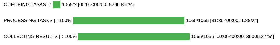
la_train_gdf.head()
la_train_gdf.shape
la_train_gdf describes 380,815 blue band AOD values that overlap with the competition training grid cells in Los Angeles!
Simple benchmark model
Using la_train_df, let's prepare an extremely simple benchmark solution for the Airathon particulate track. Keep in mind that we don't expect this model to generalize well to Taipei or Delhi since it has not seen imagery from these geographies before.
def calculate_features(
    feature_df: gpd.GeoDataFrame,
    label_df: pd.DataFrame,
    stage: str,
):
    """Given processed AOD data and training labels (train) or
    submission format (test), return a feature GeoDataFrame that contains
    features for mean, max, and min AOD.

    Args:
        feature_df (gpd.GeoDataFrame): GeoDataFrame that contains
            Points and associated values.
        label_df (pd.DataFrame): training labels (train) or
            submission format (test).
        stage (str): "train" or "test".

    Returns:
        full_data (gpd.GeoDataFrame): GeoDataFrame that contains `mean_aod`,
            `max_aod`, and `min_aod` for each grid cell and datetime.
    """
    # Add `day` column to `feature_df` and `label_df`
    feature_df["datetime"] = pd.to_datetime(
        feature_df.granule_id.str.split("_", expand=True)[0],
        format="%Y%m%dT%H:%M:%S",
        utc=True,
    )
    feature_df["day"] = feature_df.datetime.dt.date
    label_df["day"] = label_df.datetime.dt.date

    # Calculate average AOD per day/grid cell for which we have feature data
    avg_aod_day = feature_df.groupby(["day", "grid_id"]).agg(
        {"value": ["mean", "min", "max"]}
    )
    avg_aod_day.columns = ["mean_aod", "min_aod", "max_aod"]
    avg_aod_day = avg_aod_day.reset_index()

    # Join labels/submission format with feature data
    how = "inner" if stage == "train" else "left"
    full_data = pd.merge(
        label_df,
        avg_aod_day,
        how=how,
        left_on=["day", "grid_id"],
        right_on=["day", "grid_id"],
    )
    return full_data
full_data = calculate_features(la_train_gdf, train_labels, stage="train")
full_data.head(3)
We do not want to overstate our model's performance by overfitting to one or more dates or locations. To be sure that our method is sufficiently generalizable, let's set aside a portion of the data to validate the model. To ensure that we are not using data collected in the future to estimate prior PM2.5, we can subset the training data into training and validation sets using the datetime field.
# 2020 data will be held out for validation
train = full_data[full_data.datetime.dt.year <= 2019].copy()
test = full_data[full_data.datetime.dt.year > 2019].copy()
In scikit-learn, we can set up a random forest with a few lines of code.
from sklearn.ensemble import RandomForestRegressor
# Train model on train set
model = RandomForestRegressor()
model.fit(train[["mean_aod", "min_aod", "max_aod"]], train.pm25)

# Compute R2 using our holdout set
model.score(test[["mean_aod", "min_aod", "max_aod"]], test.pm25)
# Refit model on entire training set
model.fit(full_data[["mean_aod", "min_aod", "max_aod"]], full_data.pm25)
Finally, let's make predictions for the competition test set and save them to the submission format. To keep things simple, we'll impute missing features using the average, minimum, and maximum AOD values from the training data.
# Identify test granule s3 paths
test_md = pm_md[(pm_md["product"] == "maiac") & (pm_md["split"] == "test")]
# Identify test grid cells
submission_format = pd.read_csv(RAW / "submission_format.csv", parse_dates=["datetime"])
test_gc = grid_md[grid_md.index.isin(submission_format.grid_id)]
# Process test data for each location
locations = test_gc.location.unique()
loc_map = {"Delhi": "dl", "Los Angeles (SoCAB)": "la", "Taipei": "tpe"}
loc_dfs = []
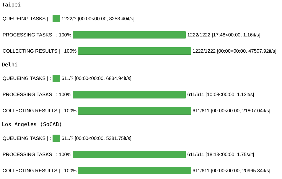
for loc in locations:
print(loc)
these_fp = list(test_md[test_md.location == loc_map[loc]].us_url)
# Create grid cell GeoDataFrame
these_grid_cells = test_gc[test_gc.location == loc]
these_polys = gpd.GeoSeries.from_wkt(these_grid_cells.wkt, crs=wgs84_crs)
these_polys.name = "geometry"
this_polys_gdf = gpd.GeoDataFrame(these_polys)
# Preprocess AOD for test granules
loc_dfs.append(preprocess_aod_47(these_fp, this_polys_gdf))
test_df = pd.concat(loc_dfs)
test_df.head(3)
# Prepare AOD features
submission_df = calculate_features(test_df, submission_format, stage="test")

# Impute missing features using training set mean/max/min
submission_df.mean_aod.fillna(la_train_gdf.value.mean(), inplace=True)
submission_df.min_aod.fillna(la_train_gdf.value.min(), inplace=True)
submission_df.max_aod.fillna(la_train_gdf.value.max(), inplace=True)
submission_df.drop(columns=["day"], inplace=True)

# Make predictions using AOD features
submission_df["preds"] = model.predict(submission_df[["mean_aod", "min_aod", "max_aod"]])
submission = submission_df[["datetime", "grid_id", "preds"]].copy()
submission.rename(columns={"preds": "value"}, inplace=True)

# Ensure submission indices match submission format
submission_format.set_index(["datetime", "grid_id"], inplace=True)
submission.set_index(["datetime", "grid_id"], inplace=True)
assert submission_format.index.equals(submission.index)
submission.head(3)
submission.describe()
Finally, we will save our submission locally.
# Save submission in the correct format
final_submission = pd.read_csv(RAW / "submission_format.csv")
final_submission["value"] = submission.reset_index().value
final_submission.to_csv((INTERIM / "submission.csv"), index=False)
We can now head to the competition submissions page and upload our submission to obtain our model's R2.

We should see an R2 of -0.0655 on the leaderboard. Lots of room for improvement! This model was only trained on data from Los Angeles and has very simple features. Now it's up to you to make improvements and increase this score. We hope this tutorial provides a helpful framework for loading and exploring the data, correcting and aligning values, and working with geospatial vector and raster data.
Head over to the challenge homepage to get started. We can't wait to see what you build!
Banner image, artist's rendering of Aqua, courtesy of NASA