Richter's Predictor - Benchmark

In this post we'll show you how to start using data science to predict the extent of earthquake damage!

Casey Fitzpatrick
DrivenData

In April of 2015 the 7.8 magnitude Gorkha earthquake occured near the Gorkha district of Gandaki Pradesh, Nepal. Almost 9,000 lives were lost, millions of people were instantly made homeless, and \$10 billion in damages––about half of Nepal's nominal GDP––were incurred. In the years since, the Nepalese government has worked intensely to help rebuild the affected districts' infrastructures. Throughout this process, the National Planning Commission, along with Kathmandu Living Labs and the Central Bureau of Statistics, has generated

One of the largest post-disaster datasets ever collected, containing valuable information on earthquake impacts, household conditions, and socio-economic-demographic statistics.

For more information, check out the [open data portal](https://opendata.klldev.org/#/).

In our brand new intermediate practice competition, your goal is to predict the level of damage a building suffered as a result of the 2015 earthquake. The data comes from the 2015 Nepal Earthquake Open Data Portal, and mainly consists of information on the buildings' structure and their legal ownership. Each row in the dataset represents a specific building in the region that was hit by Gorkha earthquake.

In this post, we'll walk through a very simple first pass model for predicting earthquake damage from structural and legal data, showing you how to load the data, make some predictions, and then submit those predictions to the competition.

To get started, we import the standard tools of the trade.

In [1]:
%matplotlib inline

from pathlib import Path

import numpy as np
import pandas as pd

import matplotlib.pyplot as plt
import seaborn as sns
In [2]:
DATA_DIR = Path('..', 'data', 'final', 'public')

Loading the Data

Destroyed temple area in Pashupatinath.

On the data download page, we provide everything you need to get started:

  • Training Values: These are the features you'll use to train a model. There are 38 features, including structual information such as the number of floors (before the earthquake), age of the building, and type of foundation, as well as legal information such as ownership status, building use, and the number of families who live there. Each building is identified by a unique (random) building_id, which you can use as an index.
  • Training Labels: These are the labels. Every building_id in the training values data has a corresponding label in this file. A 1 represents low damage, a 2 represents a medium amount of damage, and a 3 represents almost complete destruction.
  • Test Values: These are the features you'll use to make predictions after training a model. We don't give you the labels for these samples, it's up to you to generate predictions of the level of earthquake damage for these building_ids!
  • Submission Format: This gives us the filenames and columns of our submission prediction, filled with all 1 as a baseline. Your submission to the leaderboard must be in this exact form (with different prediction values, of course) in order to be scored successfully!

Since this is a benchmark, we're only going to use a subset of the features in the dataset. It's up to you to take advantage of all the information!

In [3]:
train_values = pd.read_csv(DATA_DIR / 'train_values.csv', index_col='building_id')
train_labels = pd.read_csv(DATA_DIR / 'train_labels.csv', index_col='building_id')
In [4]:
train_values.dtypes
Out[4]:
geo_level_1_id                             int64
geo_level_2_id                             int64
geo_level_3_id                             int64
count_floors_pre_eq                        int64
age                                        int64
area_percentage                            int64
height_percentage                          int64
land_surface_condition                    object
foundation_type                           object
roof_type                                 object
ground_floor_type                         object
other_floor_type                          object
position                                  object
plan_configuration                        object
has_superstructure_adobe_mud               int64
has_superstructure_mud_mortar_stone        int64
has_superstructure_stone_flag              int64
has_superstructure_cement_mortar_stone     int64
has_superstructure_mud_mortar_brick        int64
has_superstructure_cement_mortar_brick     int64
has_superstructure_timber                  int64
has_superstructure_bamboo                  int64
has_superstructure_rc_non_engineered       int64
has_superstructure_rc_engineered           int64
has_superstructure_other                   int64
legal_ownership_status                    object
count_families                             int64
has_secondary_use                          int64
has_secondary_use_agriculture              int64
has_secondary_use_hotel                    int64
has_secondary_use_rental                   int64
has_secondary_use_institution              int64
has_secondary_use_school                   int64
has_secondary_use_industry                 int64
has_secondary_use_health_post              int64
has_secondary_use_gov_office               int64
has_secondary_use_use_police               int64
has_secondary_use_other                    int64
dtype: object

Explore the Data

In [5]:
(train_labels.damage_grade
             .value_counts()
             .sort_index()
             .plot.bar(title="Number of Buildings with Each Damage Grade"))
Out[5]:
<matplotlib.axes._subplots.AxesSubplot at 0x106b1d550>
In [6]:
selected_features = ['foundation_type', 
                     'area_percentage', 
                     'height_percentage',
                     'count_floors_pre_eq',
                     'land_surface_condition',
                     'has_superstructure_cement_mortar_stone']

train_values_subset = train_values[selected_features]

A quick look at the relationships between our numeric features and labels

In [7]:
sns.pairplot(train_values_subset.join(train_labels), 
             hue='damage_grade')
Out[7]:
<seaborn.axisgrid.PairGrid at 0x1a0da806d8>

Pre-process the Data

In [8]:
train_values_subset = pd.get_dummies(train_values_subset)

The Error Metric – Micro F1

The metric for the competitions is F1 score, which balances the precision and recall of a classifier. Traditionally, the F1 score is used to evaluate performance on a binary classifier, but since we have three possible labels we will use a variant called the micro averaged F1 score.

In Python, you can easily calculate this loss using sklearn.metrics.f1_score with the keyword argument average='micro'. Here are some references that discuss the micro-averaged F1 score further:

Build the Model

This probably isn't your first data science competition (and if it is––welcome!), so you know as well as we do that random forests are often a good first model to try. We'll give random forests a shot here, and leave the stacked classifiers and deep learning models up to you.

Random Forest

In Scikit Learn, it almost couldn't be easier to grow a random forest with a fiew lines of code. We'll also show you how to throw in some mean standardization of the features and assemble it all into a pipeline.

In [9]:
# for preprocessing the data
from sklearn.preprocessing import StandardScaler

# the model
from sklearn.ensemble import RandomForestClassifier

# for combining the preprocess with model training
from sklearn.pipeline import make_pipeline

# for optimizing the hyperparameters of the pipeline
from sklearn.model_selection import GridSearchCV

The make_pipeline function automatically names the steps in your pipeline as a lowercase version of whatever the object name is.

In [10]:
pipe = make_pipeline(StandardScaler(), 
                     RandomForestClassifier(random_state=2018))
pipe
Out[10]:
Pipeline(memory=None,
     steps=[('standardscaler', StandardScaler(copy=True, with_mean=True, with_std=True)), ('randomforestclassifier', RandomForestClassifier(bootstrap=True, class_weight=None, criterion='gini',
            max_depth=None, max_features='auto', max_leaf_nodes=None,
            min_impurity_decrease=0.0, min...n_jobs=1,
            oob_score=False, random_state=2018, verbose=0,
            warm_start=False))])

From here we can easily test a few different models using GridSearchCV.

In [11]:
param_grid = {'randomforestclassifier__n_estimators': [50, 100],
              'randomforestclassifier__min_samples_leaf': [1, 5]}
gs = GridSearchCV(pipe, param_grid, cv=5)
In [12]:
gs.fit(train_values_subset, train_labels.values.ravel())
Out[12]:
GridSearchCV(cv=5, error_score='raise',
       estimator=Pipeline(memory=None,
     steps=[('standardscaler', StandardScaler(copy=True, with_mean=True, with_std=True)), ('randomforestclassifier', RandomForestClassifier(bootstrap=True, class_weight=None, criterion='gini',
            max_depth=None, max_features='auto', max_leaf_nodes=None,
            min_impurity_decrease=0.0, min...n_jobs=1,
            oob_score=False, random_state=2018, verbose=0,
            warm_start=False))]),
       fit_params=None, iid=True, n_jobs=1,
       param_grid={'randomforestclassifier__n_estimators': [50, 100], 'randomforestclassifier__min_samples_leaf': [1, 5]},
       pre_dispatch='2*n_jobs', refit=True, return_train_score='warn',
       scoring=None, verbose=0)

Take a look at the best params.

In [13]:
gs.best_params_
Out[13]:
{'randomforestclassifier__min_samples_leaf': 5,
 'randomforestclassifier__n_estimators': 100}

And the in-sample F1 micro score.

Note that we use the class predictions (.predict()), not the class probabilities (.predict_proba()).

In [14]:
from sklearn.metrics import f1_score

in_sample_preds = gs.predict(train_values_subset)
f1_score(train_labels, in_sample_preds, average='micro')
Out[14]:
0.5894259807138116

Remember, a perfect micro F1 score would be 1, so this is not a bad start given that we have 3 classes. Let's make some predictions on the test set!

Time to Predict and Submit

For the F1 Micro metric, we'll be using the class predictions, not the class probabilities. Let's load up the data, process it, and see what we get on the leaderboard.

In [15]:
test_values = pd.read_csv(DATA_DIR / 'test_values.csv', index_col='building_id')

Select the subset of features we used to train the model and create dummy variables.

In [16]:
test_values_subset = test_values[selected_features]
test_values_subset = pd.get_dummies(test_values_subset)

Make Predictions

Note that we use the class predictions, not the class probabilities.

In [17]:
predictions = gs.predict(test_values_subset)

Save Submission

We can use the column name and index from the submission format to ensure our predictions are in the form.

In [18]:
submission_format = pd.read_csv(DATA_DIR / 'submission_format.csv', index_col='building_id')
In [19]:
my_submission = pd.DataFrame(data=predictions,
                             columns=submission_format.columns,
                             index=submission_format.index)
In [20]:
my_submission.head()
Out[20]:
damage_grade
building_id
300051 3
99355 2
890251 2
745817 2
421793 2
In [21]:
my_submission.to_csv('submission.csv')

Check the head of the saved file

In [22]:
!head submission.csv
building_id,damage_grade
300051,3
99355,2
890251,2
745817,2
421793,2
871976,2
691228,2
896100,3
343471,2

Submit to leaderboard

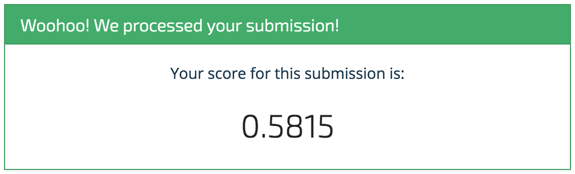
Woohoo! It's a start! And that's exactly what we intend with these benchmarks. We're sure you'll be able to top this model in no time, and we can't wait to see what you come up with. Happy importing!

Stay updated

Join our newsletter or follow us for the latest on our social impact projects, data science competitions and open source work.

There was a problem. Please try again.
Subscribe successful!
Protected by reCAPTCHA. The Google Privacy Policy and Terms of Service apply.

Latest posts

All posts

winners

Meet the winners of Phase 2 of the PREPARE Challenge

Learn about how winners detected cognitive decline using speech recordings and social determinants of health survey data

resources

Open-source packages for using speech data in ML

Overview of key open-source packages for extracting features from voice data to support ML applications

tutorial

Getting started with LLMs: a benchmark for the 'What's Up, Docs?' challenge

An introduction to using large language models via the benchmark to a document summarization challenge.

winners

Meet the Winners of the Goodnight Moon, Hello Early Literacy Screening Challenge

Learn about the results and winning methods from the early literacy screening challenge.

resources

Where to find a data job for a good cause

Finding data jobs for good causes can be difficult. Learn strategies, job lists, and tips to find organizations with open positions working on causes you care about.

winners

Meet the Winners of the Youth Mental Health Narratives Challenge

Learn about the winning solutions from the Youth Mental Health Challenge Automated Abstraction and Novel Variables Tracks

winners

Meet the winners of the Forecast and Final Prize Stages of the Water Supply Forecast Rodeo

Learn about the winners and winning solutions from the final stages of the Water Supply Forecast Rodeo.

insights

10 takeaways from 10 years of data science for social good

This year DrivenData celebrates our 10th birthday! We've spent the past decade working to use data science and AI for social good. Here are some lessons we've learned along the way.

tutorial

Goodnight Moon, Hello Early Literacy Screening Benchmark

In this guest post from the MIT Gabrieli Lab, we'll show you how to get started with the literacy screening challenge!

tutorial

Youth Mental Health: Automated Abstraction Benchmark

Learn how to process text narratives using open-source LLMs for the Youth Mental Health: Automated Abstraction challenge

winners

Meet the winners of Phase 1 of the PREPARE Challenge

Learn about the top datasets sourced for Phase 1 of the PREPARE Challenge.

resources

Teaching with DrivenData Competitions

Inspiration and resources for teaching students data science, machine learning, and AI skills with DrivenData competitions.

winners

Meet the winners of the Pose Bowl challenge

Learn about the top solutions submitted for the Pose Bowl: Spacecraft Detection and Pose Estimation Challenge.

winners

Meet the winners of the Water Supply Forecast Rodeo Hindcast Stage

Learn about the winning models for forecasting seasonal water supply from the first stage of the Water Supply Forecast Rodeo.

tools

Cookiecutter Data Science V2

Announcing the V2 release of Cookiecutter Data Science, the most widely adopted data science project template.

resources

How to make data science projects more open and inclusive

Key practices from the field of open science for making data science work more transparent, inclusive, and equitable.

winners

Meet the winners of the Kelp Wanted challenge

Dive into the solutions from the super segmenters who best detected kelp in Landsat imagery!

winners

Meet the winners of the SNOMED CT Entity Linking Challenge

Meet the winners with the best systems for detecting clinical terms in medical notes.

winners

Meet the winners of the Pale Blue Dot challenge

Learn about the top visuals created for the Pale Blue Dot: Visualization Challenge and the solvers behind them.

tutorial

NASA Pose Bowl - Benchmark

An introduction to the NASA Pose Bowl competition, with a benchmark solution for the object detection track

Work with us to build a better world

Learn more about how our team is bringing the transformative power of data science and AI to organizations tackling the world's biggest challenges.