blog

Sustainable Industry: Rinse Over Run - Benchmark


by Emily Dorne

We're really excited to launch our latest competition! In addition to an interesting, new prize structure, the subject matter is at the intersection of sustainability and industry. Improvements to these kinds of processes can have upside for both a business and the planet.

The presence of particles, bacteria, allergens, or other foreign material in a food or beverage product can put consumers at risk. Manufacturers put extra care into ensuring that equipment is properly cleaned between uses to avoid any contamination. At the same time, the cleaning processes require substantial resources in the form of time and cleaning supplies, which are often water and chemical mixtures (e.g. caustic soda, acid, etc.).

Given these concerns, the cleaning stations measure turbidity during the cleaning process. Turbidity quanitifies the suspended solids in the liquids that are coming out of the cleaning tank. The goal is to have those liquids be turbidity free, indicating that the equipment is fully clean. Depending on the expected level of turbidity, a cleaning station operator can either extend the final rinse (to eliminate remaining turbidity) or shorten it (saving time and water consumption).

The goal of this competition is to predict turbidity in the last rinsing phase in order to help minimize the use of water, energy and time, while ensuring high cleaning standards.
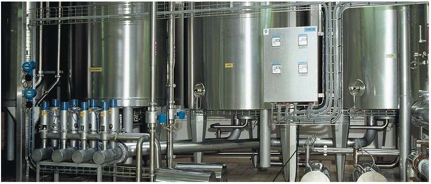
A Clean-In-Place system that is commonly used for cleaning in the food and beverage industry.

In this post, we'll walk through a very simple first pass model for predicting turbidity in the final rinse stage, showing you how to load the data, make some predictions, and then submit those predictions to the competition.

To get started, we import libraries for loading, manipulating, and visualizing the data.

In [2]:
%matplotlib inline

# mute warnings for this blog post
import warnings
warnings.filterwarnings("ignore")

from pathlib import Path

import numpy as np
import pandas as pd

pd.set_option('display.max_columns', 40)

import matplotlib.pyplot as plt

from sklearn.model_selection import train_test_split
from sklearn.ensemble import RandomForestRegressor
In [3]:
DATA_DIR = Path('../data/final/public')

Loading the data

On the data download page, we provide everything you need to get started:

  • Training Values: These are the features you'll use to train a model. There are 35 features in the data, including metadata on the cleaning process, phase, and object as well as time series data, sampled every 2 seconds. The time series measurements pertain to the monitoring and control of different cleaning process variables in both supply and return Clean-In-Place lines as well as in cleaning material tanks during the cleaning operations.

  • Training Labels: These are the labels. Every process_id in the training values data has a corresponding final_rinse_total_turbidity_liter label in this file. final_rinse_total_turbidity_liter is defined as the total quantity of turbidity returned during the target time period multiplied by the outgoing flow during the final rinsing, for each cleaning process.

  • Test Values: These are the features you'll use to make predictions after training a model. We don't give you the labels for these samples, it's up to you to generate turbidity predictions for the final rinsing phase of these processes.

  • Submission Format: This gives us the filenames and columns of our submission prediction, filled with all 1.0 as a baseline. Your submission to the leaderboard must be in this exact form (with different prediction values, of course) in order to be scored successfully!

In [4]:
# for training our model
train_values = pd.read_csv(DATA_DIR / 'train_values.csv',
                           index_col=0,
                           parse_dates=['timestamp'])

train_labels = pd.read_csv(DATA_DIR / 'train_labels.csv',
                           index_col=0)

Let's take a peek at our training features and the labels.

In [5]:
train_values.head()
Out[5]:
process_id object_id phase timestamp pipeline supply_flow supply_pressure return_temperature return_conductivity return_turbidity return_flow supply_pump supply_pre_rinse supply_caustic return_caustic supply_acid return_acid supply_clean_water return_recovery_water return_drain object_low_level tank_level_pre_rinse tank_level_caustic tank_level_acid tank_level_clean_water tank_temperature_pre_rinse tank_temperature_caustic tank_temperature_acid tank_concentration_caustic tank_concentration_acid tank_lsh_caustic tank_lsh_acid tank_lsh_clean_water tank_lsh_pre_rinse target_time_period
row_id
0 20001 405 pre_rinse 2018-04-15 04:20:47 L4 8550.348 0.615451 18.044704 4.990765 0.177228 15776.9100 True True False False False False False False True True 55.499672 41.555992 44.026875 49.474102 32.385708 83.036750 73.03241 45.394646 44.340126 False 0.0 False 0.0 False
1 20001 405 pre_rinse 2018-04-15 04:20:49 L4 11364.294 0.654297 18.229168 3.749680 0.122975 13241.4640 True True False False False False False False True True 55.487920 41.624170 44.045685 49.457645 32.385708 83.015045 73.03241 45.394447 44.339380 False 0.0 False 0.0 False
2 20001 405 pre_rinse 2018-04-15 04:20:51 L4 12174.479 0.699870 18.395544 2.783954 0.387008 10698.7850 True True False False False False False False True True 55.476166 41.638275 44.045685 49.462350 32.385708 83.015045 73.03241 45.396280 44.336735 False 0.0 False 0.0 False
3 20001 405 pre_rinse 2018-04-15 04:20:53 L4 13436.776 0.761502 18.583622 1.769353 0.213397 8007.8125 True True False False False False False False True True 55.471466 41.647675 44.048030 49.462350 32.385708 83.036750 73.03241 45.401875 44.333110 False 0.0 False 0.0 False
4 20001 405 pre_rinse 2018-04-15 04:20:55 L4 13776.766 0.837240 18.627026 0.904020 0.148293 6004.0510 True True False False False False False False True True 55.459705 41.654730 44.048030 49.462350 32.385708 83.015045 73.03241 45.398197 44.334373 False 0.0 False 0.0 False
In [6]:
train_values.dtypes
Out[6]:
process_id                             int64
object_id                              int64
phase                                 object
timestamp                     datetime64[ns]
pipeline                              object
supply_flow                          float64
supply_pressure                      float64
return_temperature                   float64
return_conductivity                  float64
return_turbidity                     float64
return_flow                          float64
supply_pump                             bool
supply_pre_rinse                        bool
supply_caustic                          bool
return_caustic                          bool
supply_acid                             bool
return_acid                             bool
supply_clean_water                      bool
return_recovery_water                   bool
return_drain                            bool
object_low_level                        bool
tank_level_pre_rinse                 float64
tank_level_caustic                   float64
tank_level_acid                      float64
tank_level_clean_water               float64
tank_temperature_pre_rinse           float64
tank_temperature_caustic             float64
tank_temperature_acid                float64
tank_concentration_caustic           float64
tank_concentration_acid              float64
tank_lsh_caustic                        bool
tank_lsh_acid                        float64
tank_lsh_clean_water                    bool
tank_lsh_pre_rinse                   float64
target_time_period                      bool
dtype: object
In [7]:
train_labels.head()
Out[7]:
final_rinse_total_turbidity_liter
process_id
20001 4.318275e+06
20002 4.375286e+05
20003 4.271977e+05
20004 7.197830e+05
20005 4.133107e+05

Explore the data

Let's get a better understanding of how the target variable is calculated by examining its components, return_turbidity and return_flow, over the target time period. The target time period is when we want to measure turbidity, and is indicated with the boolean column target_time_period. This is when we are in the final rinse and the return caustic and return acid valves have been closed for the last time.

For this exploration, we'll just look at a single cleaning process.

In [8]:
# subset to final rinse phase observations 
final_phases = train_values[(train_values.target_time_period)]

# let's look at just one process
final_phase = final_phases[final_phases.process_id == 20017]

The target variable is calculated as follows for the final rinse phase: sum(max(0, return_flow) * return_turbidity).

In [9]:
# calculate target variable
final_phase = final_phase.assign(target=np.maximum(final_phase.return_flow, 0) * final_phase.return_turbidity)

Let's plot return flow, return turbidity, and the product of the two (turbidity measured in NTU.L) side by side.

In [10]:
# plot flow, turbidity, and target 
fig, ax = plt.subplots(nrows=1, ncols=3, figsize=(20, 5))

ax[0].plot(final_phase.return_flow)
ax[0].set_title('Return flow in final phase')

ax[1].plot(final_phase.return_turbidity, c='orange')
ax[1].set_title('Return turbidity in final phase')

ax[2].plot(final_phase.target, c='green')
ax[2].set_title('Turbidity in final phase in NTU.L');

We sum over the final rinse phase to get the target value for this process, and confirm this matches the label for this process in train_labels.csv.

In [11]:
# sum to get target
final_phase.target.sum()
Out[11]:
103724.28729467509
In [12]:
# confirm that value matches the target label for this process_id
train_labels.loc[20017]
Out[12]:
final_rinse_total_turbidity_liter    103724.287295
Name: 20017, dtype: float64

Pre-process the data

Subset the data

Before doing some feature engineering, we'll want to subset our training dataset to exclude observations from the final rinse phase. The training data contains all of the available phases for reference, but the test set does not.

As per the problem description, a single object is cleaned in each process and there are five possible phases for each process:

  • Pre-rinse phase: Rinse water is pushed into the cleaning object
  • Caustic phase: Caustic soda is pushed into the cleaning object
  • Intermediate rinse phase: Clean or rinse water is pushed into the object
  • Acid phase: Nitric acid is pushed into the cleaning object
  • Final rinse phase: Clean water is pushed into the object

The test set does not include any observations from the final rinsing phase, as the goal is to predict final turbidity early enough in advance so the cleaning station operator can adjust the length of the final rinse accordingly. To ensure our model doesn't depend on observations from the final rinse phase, it's important to remove these observations from our training data.

In [13]:
train_values = train_values[train_values.phase != 'final_rinse']

In the train set, you are given all available data for each cleaning process. However, in the test set you are only given data from selected phases (up to a given time, t) and then asked to predict into the future.

  • For 10% of the test instances, t corresponds to the end of the first (pre-rinse) phase.
  • For 30% of the test instances, t corresponds to the end of the second (caustic) phase.
  • For 30% of the test instances, t corresponds to the end of the third (intermediate rinse) phase.
  • For 30% of the test instances, t corresponds to the end of the fourth (acid) phase.

To help our train set better match the test set, let's randomly drop out phases from our training set.

In [14]:
train_values.groupby('process_id').phase.nunique().value_counts().sort_index().plot.bar()
plt.title("Number of Processes with $N$ Phases");
In [15]:
# create a unique phase identifier by joining process_id and phase
train_values['process_phase'] = train_values.process_id.astype(str) + '_' + train_values.phase.astype(str)
process_phases = train_values.process_phase.unique()

# randomly select 80% of phases to keep
rng = np.random.RandomState(2019)
to_keep = rng.choice(
                process_phases,
                size=np.int(len(process_phases) * 0.8),
                replace=False)

train_limited = train_values[train_values.process_phase.isin(to_keep)]

# subset labels to match our training data
train_labels = train_labels.loc[train_limited.process_id.unique()]
In [16]:
train_limited.groupby('process_id').phase.nunique().value_counts().sort_index().plot.bar()
plt.title("Number of Processes with $N$ Phases (Subset for Training)");

Feature engineering

In train_values.csv, we have time series measurements sampled every 2 seconds, meaning we have many observations for each process. Our target variable is at the process level, so we'll want a feature matrix where each row corresponds to a unique process_id.

Since this is a benchmark, we're only going to use a subset of the variables in the dataset. It's up to you to take advantage of all the information!

First, let's create some features from the metadata about the cleaning processes. We'll create dummy variables for which pipeline the process occurs on and count the number of phases each process has.

In [17]:
def prep_metadata(df):
    # select process_id and pipeline
    meta = df[['process_id', 'pipeline']].drop_duplicates().set_index('process_id') 
    
    # convert categorical pipeline data to dummy variables
    meta = pd.get_dummies(meta)
    
    # pipeline L12 not in test data
    if 'L12' not in meta.columns:
        meta['pipeline_L12'] = 0
    
    # calculate number of phases for each process_object
    meta['num_phases'] = df.groupby('process_id')['phase'].apply(lambda x: x.nunique())
    
    return meta

# show example for first 5,000 observations
prep_metadata(train_limited.head(5000))
Out[17]:
pipeline_L3 pipeline_L4 pipeline_L7 pipeline_L12 num_phases
process_id
20001 0 1 0 0 4
20002 1 0 0 0 2
20003 1 0 0 0 3
20004 0 0 1 0 2
20005 0 0 1 0 1
20008 0 1 0 0 3

Then, we'll select the float variable measurements and calculate the following summary statistics for each:

  • minimum
  • maximum
  • mean
  • standard deviation
  • average value of the last five observations
In [18]:
# variables we'll use to create our time series features
ts_cols = [
    'process_id',
    'supply_flow',
    'supply_pressure',
    'return_temperature',
    'return_conductivity',
    'return_turbidity',
    'return_flow',
    'tank_level_pre_rinse',
    'tank_level_caustic',
    'tank_level_acid',
    'tank_level_clean_water',
    'tank_temperature_pre_rinse',
    'tank_temperature_caustic',
    'tank_temperature_acid',
    'tank_concentration_caustic',
    'tank_concentration_acid',
]
In [19]:
def prep_time_series_features(df, columns=None):
    if columns is None:
        columns = df.columns
    
    ts_df = df[ts_cols].set_index('process_id')
    
    # create features: min, max, mean, standard deviation, and mean of the last five observations
    ts_features = ts_df.groupby('process_id').agg(['min', 'max', 'mean', 'std', lambda x: x.tail(5).mean()])
    
    return ts_features

# show example for first 5,000 observations
prep_time_series_features(train_limited.head(5000), columns=ts_cols)
Out[19]:
supply_flow supply_pressure return_temperature return_conductivity ... tank_temperature_caustic tank_temperature_acid tank_concentration_caustic tank_concentration_acid
min max mean std <lambda> min max mean std <lambda> min max mean std <lambda> min max mean std <lambda> ... min max mean std <lambda> min max mean std <lambda> min max mean std <lambda> min max mean std <lambda>
process_id
20001 21.701390 59396.703 49501.604051 12445.724586 48618.3452 -0.036024 2.223741 1.673456 0.344843 1.204688 13.888889 82.530380 65.433236 22.452964 72.463108 0.255486 57.301300 32.976699 18.421732 42.254814 ... 80.768950 83.239296 82.468269 0.390909 82.870370 71.524160 73.734085 72.765519 0.365223 72.800930 44.667377 46.662950 45.266623 0.322050 45.878381 39.447857 52.411568 44.711593 0.648487 44.653038
20002 7.233796 34295.430 27142.963425 8337.197885 29688.2238 -0.034071 2.170790 1.477925 0.421852 1.552300 8.742043 76.392510 53.616841 22.887856 76.335362 0.172301 46.425180 30.834840 17.792754 42.065181 ... 80.096210 83.268234 82.305567 0.695085 82.620806 72.236690 73.397710 73.087684 0.185479 73.152490 44.773426 46.242180 45.373944 0.253696 45.269097 44.216820 44.708210 44.332388 0.079575 44.229616
20003 -1244.213000 103096.070 29902.913654 10872.426632 30179.3980 -0.033854 3.855469 2.630566 0.917518 3.092057 21.459057 81.586370 68.643926 16.976440 71.476418 0.625647 46.821130 36.146996 15.031208 43.976728 ... 80.772570 83.308014 82.409380 0.407232 82.660587 70.471640 73.328995 72.455138 0.283453 72.664208 44.209152 47.086292 45.157076 0.296316 44.669835 43.750900 45.270653 44.503377 0.236661 44.716846
20004 -43.402780 49537.035 31117.193119 13046.723480 33796.2958 -0.009549 0.482422 0.287865 0.163790 0.343012 10.854311 82.107200 58.645540 21.843451 71.589264 0.198415 46.577435 29.147263 18.143533 44.471240 ... 81.474250 83.268234 82.498877 0.442668 82.852287 71.885850 73.354310 72.722285 0.243813 72.655524 44.831688 46.164917 45.176648 0.172123 45.225381 44.154810 45.862520 44.835026 0.485012 45.226021
20005 0.000000 31295.209 28241.716353 7107.794924 30962.0944 -0.023438 0.487196 0.418469 0.128794 0.468186 17.986834 71.520546 58.049278 19.047244 70.915075 0.297533 50.747000 33.776595 18.339520 42.345008 ... 82.103584 83.112700 82.697856 0.249261 82.240306 71.983505 73.350690 72.674948 0.353317 73.107639 44.638810 46.644493 45.163984 0.471708 45.739765 43.527600 44.412254 43.921479 0.249111 43.952939
20008 28638.598000 60980.902 51773.149642 8205.815088 55064.3812 -0.092665 0.174913 0.167884 0.036967 0.135851 12.803820 82.837820 76.165141 16.802885 28.678385 1.070271 53.216606 40.437314 11.592061 48.014119 ... 81.929980 83.405670 82.602451 0.281236 82.223670 72.406685 72.656250 72.552770 0.055230 72.526038 44.786827 47.464478 45.379996 0.385137 45.343967 44.693570 48.434254 44.821386 0.331357 44.948764

6 rows × 75 columns

Let's write a simple function to aggregate all this feature engineering.

In [20]:
def create_feature_matrix(df):
    metadata = prep_metadata(df)
    time_series = prep_time_series_features(df)
    
    # join metadata and time series features into a single dataframe
    feature_matrix = pd.concat([metadata, time_series], axis=1)
    
    return feature_matrix
In [21]:
train_features = create_feature_matrix(train_limited)
In [22]:
train_features.head()
Out[22]:
pipeline_L1 pipeline_L10 pipeline_L11 pipeline_L12 pipeline_L2 pipeline_L3 pipeline_L4 pipeline_L6 pipeline_L7 pipeline_L8 pipeline_L9 num_phases (supply_flow, min) (supply_flow, max) (supply_flow, mean) (supply_flow, std) (supply_flow, <lambda>) (supply_pressure, min) (supply_pressure, max) (supply_pressure, mean) ... (tank_temperature_caustic, min) (tank_temperature_caustic, max) (tank_temperature_caustic, mean) (tank_temperature_caustic, std) (tank_temperature_caustic, <lambda>) (tank_temperature_acid, min) (tank_temperature_acid, max) (tank_temperature_acid, mean) (tank_temperature_acid, std) (tank_temperature_acid, <lambda>) (tank_concentration_caustic, min) (tank_concentration_caustic, max) (tank_concentration_caustic, mean) (tank_concentration_caustic, std) (tank_concentration_caustic, <lambda>) (tank_concentration_acid, min) (tank_concentration_acid, max) (tank_concentration_acid, mean) (tank_concentration_acid, std) (tank_concentration_acid, <lambda>)
process_id
20001 0 0 0 0 0 0 1 0 0 0 0 4 21.701390 59396.703 49501.604051 12445.724586 48618.3452 -0.036024 2.223741 1.673456 ... 80.768950 83.239296 82.468269 0.390909 82.870370 71.524160 73.734085 72.765519 0.365223 72.800930 44.667377 46.662950 45.266623 0.322050 45.878381 39.447857 52.411568 44.711593 0.648487 44.653038
20002 0 0 0 0 0 1 0 0 0 0 0 2 7.233796 34295.430 27142.963425 8337.197885 29688.2238 -0.034071 2.170790 1.477925 ... 80.096210 83.268234 82.305567 0.695085 82.620806 72.236690 73.397710 73.087684 0.185479 73.152490 44.773426 46.242180 45.373944 0.253696 45.269097 44.216820 44.708210 44.332388 0.079575 44.229616
20003 0 0 0 0 0 1 0 0 0 0 0 3 -1244.213000 103096.070 29902.913654 10872.426632 30179.3980 -0.033854 3.855469 2.630566 ... 80.772570 83.308014 82.409380 0.407232 82.660587 70.471640 73.328995 72.455138 0.283453 72.664208 44.209152 47.086292 45.157076 0.296316 44.669835 43.750900 45.270653 44.503377 0.236661 44.716846
20004 0 0 0 0 0 0 0 0 1 0 0 2 -43.402780 49537.035 31117.193119 13046.723480 33796.2958 -0.009549 0.482422 0.287865 ... 81.474250 83.268234 82.498877 0.442668 82.852287 71.885850 73.354310 72.722285 0.243813 72.655524 44.831688 46.164917 45.176648 0.172123 45.225381 44.154810 45.862520 44.835026 0.485012 45.226021
20005 0 0 0 0 0 0 0 0 1 0 0 1 0.000000 31295.209 28241.716353 7107.794924 30962.0944 -0.023438 0.487196 0.418469 ... 82.103584 83.112700 82.697856 0.249261 82.240306 71.983505 73.350690 72.674948 0.353317 73.107639 44.638810 46.644493 45.163984 0.471708 45.739765 43.527600 44.412254 43.921479 0.249111 43.952939

5 rows × 87 columns

The error metric

The metric for this competition is mean adjusted absolute error, which captures how much the predicted value of turbidity in the final rinse phase differs from the actual value. These percent differences are then averaged across all cleaning processes to get a final score.

See the competition problem description page for more info on the metric!

Build the model

Now that we have our process level features, we're ready to train a model. Random forests are often a good model to try first, especially when we have numeric and categorical variables in our feature space. scikit-learn makes this quick and easy.

In [23]:
%%time
rf = RandomForestRegressor(n_estimators=1000, random_state=2019)
rf.fit(train_features, np.ravel(train_labels))
CPU times: user 5min 29s, sys: 1.91 s, total: 5min 31s
Wall time: 5min 32s

Time to predict and submit

Let's load up the test data, generate our features, and see how well we score on the leaderboard.

In [24]:
# load the test data
test_values = pd.read_csv(DATA_DIR / 'test_values.csv',
                         index_col=0,
                         parse_dates=['timestamp'])
In [25]:
# create metadata and time series features
test_features = create_feature_matrix(test_values)
In [26]:
test_features.head()
Out[26]:
pipeline_L1 pipeline_L10 pipeline_L11 pipeline_L2 pipeline_L3 pipeline_L4 pipeline_L6 pipeline_L7 pipeline_L8 pipeline_L9 pipeline_L12 num_phases (supply_flow, min) (supply_flow, max) (supply_flow, mean) (supply_flow, std) (supply_flow, <lambda>) (supply_pressure, min) (supply_pressure, max) (supply_pressure, mean) ... (tank_temperature_caustic, min) (tank_temperature_caustic, max) (tank_temperature_caustic, mean) (tank_temperature_caustic, std) (tank_temperature_caustic, <lambda>) (tank_temperature_acid, min) (tank_temperature_acid, max) (tank_temperature_acid, mean) (tank_temperature_acid, std) (tank_temperature_acid, <lambda>) (tank_concentration_caustic, min) (tank_concentration_caustic, max) (tank_concentration_caustic, mean) (tank_concentration_caustic, std) (tank_concentration_caustic, <lambda>) (tank_concentration_acid, min) (tank_concentration_acid, max) (tank_concentration_acid, mean) (tank_concentration_acid, std) (tank_concentration_acid, <lambda>)
process_id
20000 0 0 0 0 0 1 0 0 0 0 0 2 14.467592 35966.434 27807.728660 13583.904151 34307.0026 -0.036024 2.685981 1.876977 ... 79.734520 83.195890 82.309278 0.861146 82.319154 71.86415 72.92028 72.609589 0.218346 72.858795 44.521880 46.734280 45.359978 0.263476 45.360349 44.753242 45.244890 45.070216 0.069214 45.050809
20006 0 0 0 0 0 0 1 0 0 0 0 2 30.743633 28443.285 16258.187723 6882.667095 19974.6816 -0.037543 0.597873 0.435473 ... 81.517650 83.033134 82.486534 0.467442 82.472513 71.05758 73.44112 72.284690 0.386755 72.006654 44.463470 46.812943 45.265983 0.309268 45.244624 44.253990 47.871460 45.552704 0.902801 45.186858
20007 0 0 0 0 0 0 1 0 0 0 0 3 32.552086 25936.777 13532.733464 8759.422248 20006.1486 -0.037543 0.456380 0.223662 ... 82.118060 83.271840 82.704190 0.359573 82.982490 72.17882 73.46282 72.628118 0.197237 72.649013 45.257053 45.813564 45.479250 0.098108 45.488373 43.918640 44.796196 44.505637 0.263041 44.244708
20009 0 0 0 0 0 1 0 0 0 0 0 3 -1236.979200 103153.930 30343.165310 17312.277417 36157.4072 -0.035807 2.739583 1.629695 ... 81.922745 83.152490 82.545086 0.231431 82.638890 71.06843 72.60200 72.388596 0.240142 72.305414 44.548534 46.639267 45.179930 0.367397 44.965748 44.475380 45.165077 44.602441 0.247910 45.163842
20010 0 0 0 0 0 0 0 1 0 0 0 4 0.000000 50057.867 31817.032332 11812.419165 32910.8792 -0.035373 0.579427 0.310861 ... 80.457900 83.203125 82.292013 0.662845 82.582466 71.19141 73.38686 72.461240 0.294193 72.743060 43.544760 47.820510 45.347678 0.439164 44.925080 44.013447 47.362960 44.911785 0.648652 44.414867

5 rows × 87 columns

Make predictions

We call the predict method on our model to generate a prediction for each process.

In [27]:
preds = rf.predict(test_features)

Save submission

In order for our submission to be evaluated successfully, it needs to exactly match the format of submission_format.csv. We can use the column name and index from the submission format to ensure our predictions are in the correct format.

In [28]:
submission_format = pd.read_csv(DATA_DIR / 'submission_format.csv', index_col=0)
In [29]:
# confirm everything is in the right order
assert np.all(test_features.index == submission_format.index)
In [30]:
my_submission = pd.DataFrame(data=preds,
                             columns=submission_format.columns,
                             index=submission_format.index)
In [31]:
my_submission.head()
Out[31]:
final_rinse_total_turbidity_liter
process_id
20000 1.003440e+06
20006 1.261752e+06
20007 1.313289e+06
20009 1.793753e+06
20010 7.934597e+05
In [32]:
my_submission.to_csv('submission.csv')

Check the head of the saved file.

In [33]:
!head submission.csv
process_id,final_rinse_total_turbidity_liter
20000,1003440.3019991388
20006,1261751.686181902
20007,1313288.972602507
20009,1793753.4025422381
20010,793459.7421908235
20012,680657.6576431732
20013,128615.7840860363
20015,1073651.217858319
20020,817669.8233567851

Looks good, let's send it off!

Submit to leaderboard

Woohoo! It's a start! And that's exactly what we intend with these benchmarks. We're sure you'll be able to top this model in no time, and we can't wait to see what you come up with. Happy importing!