How to Predict Harmful Algal Blooms Using LightGBM and Satellite Imagery¶

Welcome to the benchmark notebook for the Tick Tick Bloom: Harmful Algal Bloom Detection Challenge! If you are just getting starting, we recommended reading the competition homepage first. The goal of this benchmark is to:

Demonstrate how to explore and work with the data
Provide a basic framework for building a model
Demonstrate how to package your work correctly for submission

You can either expand on and improve this benchmark, or start with something completely different! Let's get started.

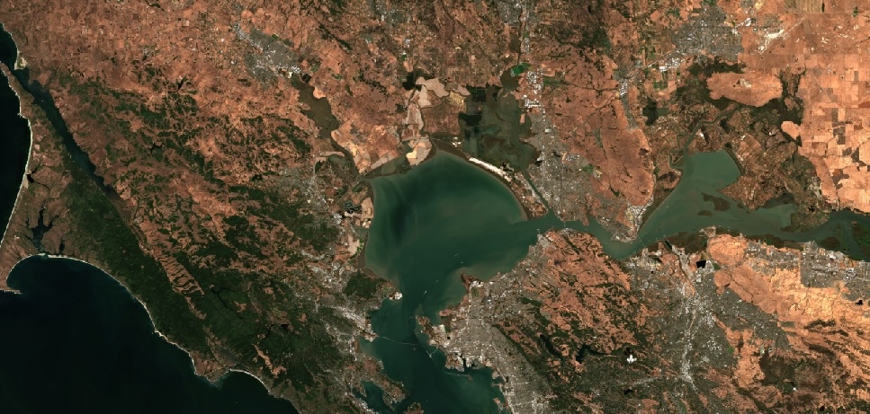
Inland water bodies like lakes and reservoirs provide critical drinking water and recreation for communities, and habitats for marine life. A significant challenge that water quality managers face is the formation of harmful algal blooms (HABs) such as cyanobacteria. HABs produce toxins that are poisonous to humans and their pets, and threaten marine ecosystems by blocking sunlight and oxygen. Manual water sampling, or “in situ” sampling, is generally used to monitor cyanobacteria in inland water bodies. In situ sampling is accurate, but time intensive and difficult to perform continuously.

Your goal in this challenge is to use satellite imagery to detect and classify the severity of cyanobacteria blooms in small, inland water bodies like reservoirs. Ultimately, better awareness of algal blooms helps keep both the human and marine life that relies on these water bodies safe and healthy.

In this post, we'll cover:¶

Exploring the data
Pulling and processing feature data from Sentinel-2 L2A and Landsat Level-2 using the Planetary Computer
Building a tree-based model using LightGBM
Generating a properly formatted submission

In [1]:

%load_ext lab_black
%load_ext autoreload
%autoreload 2

In [2]:

import cv2
from datetime import timedelta
import matplotlib.pyplot as plt
import numpy as np
import odc.stac
import pandas as pd
from pathlib import Path
from sklearn.metrics import mean_squared_error
from sklearn.preprocessing import StandardScaler
from tqdm import tqdm

%matplotlib inline

First, we'll download all of the competition data to a local folder.

The contents of the data folder are:

.
├── metadata.csv
├── submission_format.csv
└── train_labels.csv

In [3]:

DATA_DIR = Path.cwd().parent.resolve() / "data/final/public"
assert DATA_DIR.exists()

Explore the data¶

Labels in this competition are based on “in situ” samples that were collected manually and then analyzed for cyanobacteria density. Each measurement is a unique combination of date and location (latitude and longitude).

`metadata.csv`¶

metadata.csv includes all of the sample measurements in the data. It has the following columns:

uid (str): unique ID for each row. Each row is a unique combination of date and location (latitude and longitude).
date (pd.datetime): date when the sample was collected, in the format YYYY-MM-DD
latitude (float): latitude of the location where the sample was collected
longitude (float): longitude of the location where the sample was collected
region (str): region of the US. This will be used in scoring to calculate region-specific RMSEs. Final score will be the average across the four US regions.
split (str): indicates whether the row is part of the train set or the test set. Metadata is provided for all points in the train and test sets.

The geographic points in the train and test sets are distinct. This means that none of the test set points are also in the train set, so your model's performance will be measured on unseen locations.

The main feature data for this competition is satellite imagery from Sentinel-2 and Landsat. Participants will access all feature data through external, publicly available APIs. Relevant imagery can be identified using the location and date of each sample from the metadata.

For a more detailed description of the competition data, see the Problem Description page.

In [4]:

metadata = pd.read_csv(DATA_DIR / "metadata.csv")
metadata.head()

Out[4]:

	uid	latitude	longitude	date	split
0	aabm	39.080319	-86.430867	2018-05-14	train
1	aabn	36.559700	-121.510000	2016-08-31	test
2	aacd	35.875083	-78.878434	2020-11-19	train
3	aaee	35.487000	-79.062133	2016-08-24	train
4	aaff	38.049471	-99.827001	2019-07-23	train

In [5]:

metadata.split.value_counts(dropna=False)

Out[5]:

train    17060
test      6510
Name: split, dtype: int64

Location

Let's take a look at the distribution of samples by location.

In [6]:

import geopandas as gpd
from shapely.geometry import Point

# load the default geopandas base map file to plot points on
world = gpd.read_file(gpd.datasets.get_path("naturalearth_lowres"))

In [7]:

fig, ax = plt.subplots(figsize=(9, 4))

# map the training data
base = world[world.name == "United States of America"].plot(
    edgecolor="gray", color="ghostwhite", figsize=(9, 4), alpha=0.3, ax=ax
)
train_meta = metadata[metadata["split"] == "train"]
geometry = [Point(xy) for xy in zip(train_meta["longitude"], train_meta["latitude"])]
gdf = gpd.GeoDataFrame(train_meta, geometry=geometry)
gdf.plot(ax=base, marker=".", markersize=3, color="blue", label="Train", alpha=0.6)

# map the test data
test_meta = metadata[metadata["split"] == "test"]
geometry = [Point(xy) for xy in zip(test_meta["longitude"], test_meta["latitude"])]
gdf = gpd.GeoDataFrame(test_meta, geometry=geometry)
gdf.plot(ax=base, marker=".", markersize=3, color="orange", label="Test", alpha=0.6)

plt.xlabel("Longitude")
plt.ylabel("Latitude")
plt.xlim([-125, -65])
plt.ylim([25, 50])
plt.legend(loc=4, markerscale=3)

Out[7]:

<matplotlib.legend.Legend at 0x7f7ed7562c10>

We can see that the sampling points are distributed all throughout the continental United States.

Date

What date range are the samples from?

In [8]:

# convert date to pd.datetime
metadata.date = pd.to_datetime(metadata.date)

# what is the date range?
metadata.groupby("split").agg(min_date=("date", min), max_date=("date", max))

Out[8]:

	min_date	max_date
split
test	2013-01-08	2021-12-29
train	2013-01-04	2021-12-14

In [9]:

# what years are in the data?
pd.crosstab(metadata.date.dt.year, metadata.split).plot(kind="bar")
plt.ylabel("Number of samples")
plt.xlabel("Year")
plt.title("Distribution of years in the data")

Out[9]:

Text(0.5, 1.0, 'Distribution of years in the data')

In [10]:

# what seasons are the data points from?
metadata["season"] = (
    metadata.date.dt.month.replace([12, 1, 2], "winter")
    .replace([3, 4, 5], "spring")
    .replace([6, 7, 8], "summer")
    .replace([9, 10, 11], "fall")
)
metadata.season.value_counts()

Out[10]:

summer    10813
spring     5045
fall       4758
winter     2954
Name: season, dtype: int64

Most of the data is from summer. Harmful algal blooms are more likely to be dangerous during the summer because more individuals are taking advantage of water bodies like lakes for recreation.

In [11]:

# where is data from for each season?
fig, axes = plt.subplots(2, 2, figsize=(10, 5))

for season, ax in zip(metadata.season.unique(), axes.flatten()):
    base = world[world.name == "United States of America"].plot(
        edgecolor="gray", color="ghostwhite", alpha=0.3, ax=ax
    )

    sub = metadata[metadata.season == season]
    geometry = [Point(xy) for xy in zip(sub["longitude"], sub["latitude"])]
    gdf = gpd.GeoDataFrame(sub, geometry=geometry)
    gdf.plot(ax=base, marker=".", markersize=2.5)
    ax.set_xlim([-125, -66])
    ax.set_ylim([25, 50])
    ax.set_title(f"{season.capitalize()} data points")
    ax.axis("off")

`train_labels.csv`¶

Let's look at the labels for the training data.

In [12]:

train_labels = pd.read_csv(DATA_DIR / "train_labels.csv")
train_labels.head()

Out[12]:

	uid	region	severity	density
0	aabm	midwest	1	585.0
1	aacd	south	1	290.0
2	aaee	south	1	1614.0
3	aaff	midwest	3	111825.0
4	aafl	midwest	4	2017313.0

In [13]:

train_labels.shape

Out[13]:

(17060, 4)

We have one row per in situ sample. Each row is a unique combination of date and location (latitude + longitude). There are columns for:

uid (str): unique ID for each row. The uid maps each row in train_labels.csv to metadata.csv
region (str): US region in which the sample was taken. Scores are calculated separately for each of these regions, and then averaged. See the Problem Description page for details.
severity (int): severity level based on the cyanobacteria density. This is what you'll be predicting.
density (float): raw measurement of total cyanobacteria density in cells per milliliter (mL)

Note that the target value for participants to predict a severity level, NOT raw cell density in cells per mL. The severity levels are:

`severity`	Density range (cells per mL)
1	<20,000
2	20,000 - <100,000
3	100,000 - <1,000,000
4	1,000,000 - <10,000,000
5	≥10,000,000

We can find the matching metadata for each training label by merging on uid. For example:

train_labels_and_metadata = train_labels.merge(
    metadata, how="left", left_on="uid", right_on="uid", validate="1:1"
)

Cyanobacteria values

What are the cyanobacteria severity values like?

In [14]:

severity_counts = (
    train_labels.replace(
        {
            "severity": {
                1: "1 (<20,000)",
                2: "2 (20,000-100,000)",
                3: "3 (100,000 - 1,000,000)",
                4: "4 (1,00,000 - 10,000,000)",
                5: "5 (>10,000,00)",
            }
        }
    )
    .severity.value_counts()
    .sort_index(ascending=False)
)
plt.barh(severity_counts.index, severity_counts.values)
plt.xlabel("Number of samples")
plt.ylabel("Severity (range in cells/mL)")
plt.title("Train labels severity level counts")

Out[14]:

Text(0.5, 1.0, 'Train labels severity level counts')

In [15]:

train_labels.density.describe()

Out[15]:

count    1.706000e+04
mean     1.074537e+06
std      6.836693e+06
min      0.000000e+00
25%      4.066000e+03
50%      3.270975e+04
75%      4.849192e+05
max      8.046675e+08
Name: density, dtype: float64

We can see that the density is highly skewed to the right, with a long tail of very high values.

There are also some rows where the density of cyanobacteria is 0.

In [16]:

(train_labels.density == 0).sum()

Out[16]:

`submission_format.csv`¶

Now let's look at the submission format. To create your own submission, download the submission format and replace the severity column with your own prediction values. To be scored correctly, the order of your predictions must match the order of uids in the submission format.

In [17]:

submission_format = pd.read_csv(DATA_DIR / "submission_format.csv", index_col=0)
submission_format.head()

Out[17]:

	region	severity
uid
aabn	west	1
aair	west	1
aajw	northeast	1
aalr	midwest	1
aalw	west	1

In [18]:

submission_format.shape

Out[18]:

(6510, 2)

Like the training data, each row is a unique combination of location and date. The columns in submission_format.csv are:

uid (str): unique ID for each row. The uid maps each row in train_labels.csv to metadata.csv
region (str): US region in which the sample was taken. Scores are calculated separately for each of these regions, and then averaged. See the Problem Description page for details.
severity (int): placeholder for severity level based on the cyanobacteria density - all values are 0. This is the column that you will replace with your own predictions to create a submission. Participants should submit predictions for severity level, NOT for the raw cell density value in cells per mL.

Process feature data¶

Feature data is not provided through the competition site. Instead, participants will access all feature data through external, publicly available APIs. Relevant imagery can be identified using the location and date of each sample, listed in metadata.csv.

In this section, we'll walk through the process of pulling in matching satellite imagery using Microsoft's Planetary Computer. We'll only use Sentinel-2 L2A and Landsat Level-2 satellite imagery. Sentinel-2 L1C and Landsat Level-1 imagery are also allowed. For links to more guides on how to pull feature data, see the Problem Description page. There are a number of optional sources in addition to satellite imagery that you can also experiment with!

The general steps we'll use to pull satellite data are:

Establish a connection to the Planetary Computer's STAC API using the planetary_computer and pystac_client Python packages.
Query the STAC API for scenes that capture our in situ labels. For each sample, we'll search for imagery that includes the sample's location (latitude and longitude) around the date the sample was taken. In this benchmark, we'll use only Sentinel-2 L2A and Landsat Level-2 data.
Select one image for each sample. We'll use Sentinel-2 data wherever it is available, because it is higher resolution. We'll have to use Landsat for data before roughly 2016, because Sentinel-2 was not available yet.
Convert the image to a 1-dimensional list of features that can be input into our tree model

We'll first walk through these steps for just one example measurement. Then, we'll refactor the process and run it on all of our metadata.

In [19]:

# Establish a connection to the STAC API
import planetary_computer as pc
from pystac_client import Client

catalog = Client.open(
    "https://planetarycomputer.microsoft.com/api/stac/v1", modifier=pc.sign_inplace
)

Walk through pulling feature data for one sample¶

Query the STAC API¶

In [20]:

example_row = metadata[metadata.uid == "garm"].iloc[0]
example_row

Out[20]:

uid                         garm
latitude                41.98006
longitude             -110.65734
date         2021-09-27 00:00:00
split                      train
season                      fall
Name: 5461, dtype: object

We can search (41.98006, -110.65734) in Google maps to see example where this sample is from. Turns out it's from Lake Viva Naughton in Wyoming!

Location range: We'll search an area with 50,000 meters on our either side of our sample point (100,000 m x 100,000 m), to make sure we're pulling in all relevant imagery. This is just a starting point, and you can improve on how to best search for the correct location in the Planetary Computer.

In [21]:

import geopy.distance as distance

In [22]:

# get our bounding box to search latitude and longitude coordinates
def get_bounding_box(latitude, longitude, meter_buffer=50000):
    """
    Given a latitude, longitude, and buffer in meters, returns a bounding
    box around the point with the buffer on the left, right, top, and bottom.

    Returns a list of [minx, miny, maxx, maxy]
    """
    distance_search = distance.distance(meters=meter_buffer)

    # calculate the lat/long bounds based on ground distance
    # bearings are cardinal directions to move (south, west, north, and east)
    min_lat = distance_search.destination((latitude, longitude), bearing=180)[0]
    min_long = distance_search.destination((latitude, longitude), bearing=270)[1]
    max_lat = distance_search.destination((latitude, longitude), bearing=0)[0]
    max_long = distance_search.destination((latitude, longitude), bearing=90)[1]

    return [min_long, min_lat, max_long, max_lat]


bbox = get_bounding_box(example_row.latitude, example_row.longitude, meter_buffer=50000)
bbox

Out[22]:

[-111.26063646639783,
 41.52988747516146,
 -110.05404353360218,
 42.43019710235757]

Time range: We want our feature data to be as close to the time of the sample as possible, because in algal blooms in small water bodies form and move very rapidly. Remember, you cannot use any data collected after the date of the sample.

Imagery taken with roughly 10 days of the sample will generally still be an accurate representation of environmental conditions at the time of the sample. For some data points you may not be able to get data within 10 days, and may have to use earlier data. We'll search the fifteen days up to the sample time, including the sample date.

In [23]:

# get our date range to search, and format correctly for query
def get_date_range(date, time_buffer_days=15):
    """Get a date range to search for in the planetary computer based
    on a sample's date. The time range will include the sample date
    and time_buffer_days days prior

    Returns a string"""
    datetime_format = "%Y-%m-%dT"
    range_start = pd.to_datetime(date) - timedelta(days=time_buffer_days)
    date_range = f"{range_start.strftime(datetime_format)}/{pd.to_datetime(date).strftime(datetime_format)}"

    return date_range


date_range = get_date_range(example_row.date)
date_range

Out[23]:

'2021-09-12T/2021-09-27T'

In [24]:

# search the planetary computer sentinel-l2a and landsat level-2 collections
search = catalog.search(
    collections=["sentinel-2-l2a", "landsat-c2-l2"], bbox=bbox, datetime=date_range
)

# see how many items were returned
items = [item for item in search.get_all_items()]
len(items)

Out[24]:

Select one image¶

The planetary computer returned 46 different items! Let's look at some of the details of the items that were found to match our label.

Remember that our example measurement was taken on 2021-09-27 at coordinates (41.98006, -110.65734). Because we used a bounding box around the sample to search, the Planetary Computer returned all items that contain any part of that bounding box. This means we still have to double check whether each item actually contains our sample point.

In [25]:

# get details of all of the items returned
item_details = pd.DataFrame(
    [
        {
            "datetime": item.datetime.strftime("%Y-%m-%d"),
            "platform": item.properties["platform"],
            "min_long": item.bbox[0],
            "max_long": item.bbox[2],
            "min_lat": item.bbox[1],
            "max_lat": item.bbox[3],
            "bbox": item.bbox,
            "item_obj": item,
        }
        for item in items
    ]
)

# check which rows actually contain the sample location
item_details["contains_sample_point"] = (
    (item_details.min_lat < example_row.latitude)
    & (item_details.max_lat > example_row.latitude)
    & (item_details.min_long < example_row.longitude)
    & (item_details.max_long > example_row.longitude)
)

print(
    f"Filtering from {len(item_details)} returned to {item_details.contains_sample_point.sum()} items that contain the sample location"
)

item_details = item_details[item_details["contains_sample_point"]]
item_details[["datetime", "platform", "contains_sample_point", "bbox"]].sort_values(
    by="datetime"
)

Filtering from 46 returned to 7 items that contain the sample location

Out[25]:

	datetime	platform	contains_sample_point	bbox
44	2021-09-12	landsat-8	True	[-111.34023745, 40.67702495, -108.51528663, 42...
34	2021-09-14	Sentinel-2A	True	[-111.000244, 41.45624189757688, -109.665115, ...
21	2021-09-19	Sentinel-2B	True	[-111.000244, 41.45624189757688, -109.665115, ...
26	2021-09-19	landsat-8	True	[-112.92522743, 40.67353498, -110.06644659, 42...
18	2021-09-20	landsat-7	True	[-111.60018779, 40.80284495, -108.59831681, 42...
8	2021-09-24	Sentinel-2A	True	[-111.000244, 41.4562419, -109.665115, 42.4526...
5	2021-09-27	landsat-7	True	[-113.18385774, 40.78803499, -110.15150674, 42...

To keep things simple in this benchmark, we'll just choose one to input into our benchmark model. Note that in your solution, you could find a way to incorporate multiple images!

We'll narrow to one image in two steps:

If any Sentinel imagery is available, filter to only Sentinel imagery. Sentinel-2 is higher resolution than Landsat, which is extremely helpful for blooms in small water bodies. In this case, two images are from Sentinel and contain the actual sample location.
Select the item that is the closest time wise to the sampling date. This gives us a Sentinel-2A item that was captured on 10/20/2022 - two days before our sample was collected on 10/22.

This is a very simple way to choose the best image. You may want to explore additional strategies like selecting an image with less cloud cover obscuring the Earth's surface (as in this tutorial).

In [26]:

# 1 - filter to sentinel
item_details[item_details.platform.str.contains("Sentinel")]

Out[26]:

	datetime	platform	min_long	max_long	min_lat	max_lat	bbox	item_obj	contains_sample_point
8	2021-09-24	Sentinel-2A	-111.000244	-109.665115	41.456242	42.452691	[-111.000244, 41.4562419, -109.665115, 42.4526...	<Item id=S2A_MSIL2A_20210924T181101_R084_T12TW...	True
21	2021-09-19	Sentinel-2B	-111.000244	-109.665115	41.456242	42.452691	[-111.000244, 41.45624189757688, -109.665115, ...	<Item id=S2B_MSIL2A_20210919T180919_R084_T12TW...	True
34	2021-09-14	Sentinel-2A	-111.000244	-109.665115	41.456242	42.452691	[-111.000244, 41.45624189757688, -109.665115, ...	<Item id=S2A_MSIL2A_20210914T180951_R084_T12TW...	True

In [27]:

# 2 - take closest by date
best_item = (
    item_details[item_details.platform.str.contains("Sentinel")]
    .sort_values(by="datetime", ascending=False)
    .iloc[0]
)
best_item

Out[27]:

datetime                                                        2021-09-24
platform                                                       Sentinel-2A
min_long                                                       -111.000244
max_long                                                       -109.665115
min_lat                                                          41.456242
max_lat                                                          42.452691
bbox                     [-111.000244, 41.4562419, -109.665115, 42.4526...
item_obj                 <Item id=S2A_MSIL2A_20210924T181101_R084_T12TW...
contains_sample_point                                                 True
Name: 8, dtype: object

This gives us a Sentinel-2A item that was captured on 9/24/2021 -- three days before our sample was collected on 9/27/2021.

In [28]:

item = best_item.item_obj

This item comes with a number of "assets". Let's see what these are.

In [29]:

# What assets are available?
for asset_key, asset in item.assets.items():
    print(f"{asset_key:<25} - {asset.title}")

AOT                       - Aerosol optical thickness (AOT)
B01                       - Band 1 - Coastal aerosol - 60m
B02                       - Band 2 - Blue - 10m
B03                       - Band 3 - Green - 10m
B04                       - Band 4 - Red - 10m
B05                       - Band 5 - Vegetation red edge 1 - 20m
B06                       - Band 6 - Vegetation red edge 2 - 20m
B07                       - Band 7 - Vegetation red edge 3 - 20m
B08                       - Band 8 - NIR - 10m
B09                       - Band 9 - Water vapor - 60m
B11                       - Band 11 - SWIR (1.6) - 20m
B12                       - Band 12 - SWIR (2.2) - 20m
B8A                       - Band 8A - Vegetation red edge 4 - 20m
SCL                       - Scene classfication map (SCL)
WVP                       - Water vapour (WVP)
visual                    - True color image
preview                   - Thumbnail
safe-manifest             - SAFE manifest
granule-metadata          - Granule metadata
inspire-metadata          - INSPIRE metadata
product-metadata          - Product metadata
datastrip-metadata        - Datastrip metadata
tilejson                  - TileJSON with default rendering
rendered_preview          - Rendered preview

We have visible bands (red, green, and blue), as well as a number of other spectral ranges and a few algorithmic bands. The Sentinel-2 mission guide has more details about what these bands are and how to use them!

A few of the algorithmic bands that may be useful are:

Scene classification (SCL): The scene classification band sorts pixels into categories including water, high cloud probability, medium cloud probability, and vegetation. Water pixels could be used to calculate the size of a given water body, which impacts the behavior of blooms. Vegetation can indicate non-toxic marine life like sea grass that sometimes resembles cyanobacteria.
Cloud masks (CLM): Sentinel-2’s cloud bands can be used to filter out cloudy pixels. Pixels that are obscured by clouds are likely not helpful for algal bloom detection because the actual water surface is not captured.

We won't explore these in the benchmark, but you can go wild in your solution!

Visualizing Sentinel-2 imagery¶

Let's see what the imagery actually looks like.

In [30]:

import rioxarray
from IPython.display import Image
from PIL import Image as PILImage

In [31]:

# see the whole image
img = Image(url=item.assets["rendered_preview"].href, width=500)

Image(url=item.assets["rendered_preview"].href, width=500)

Out[31]:

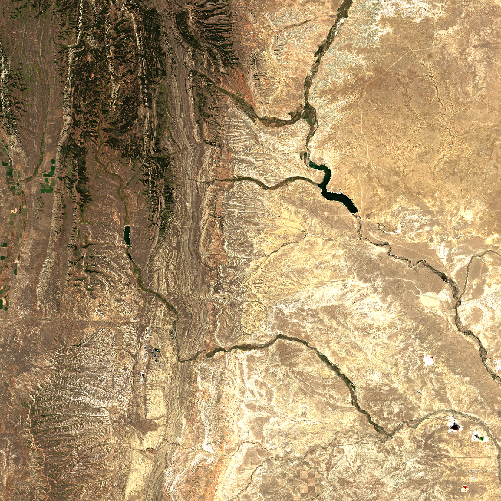
That's a LOT of area, and all we care about is right around our sampling point. Let's get a closer to look to make sure we're in the right neighborhood.

In [32]:

def crop_sentinel_image(item, bounding_box):
    """
    Given a STAC item from Sentinel-2 and a bounding box tuple in the format
    (minx, miny, maxx, maxy), return a cropped portion of the item's visual
    imagery in the bounding box.

    Returns the image as a numpy array with dimensions (color band, height, width)
    """
    (minx, miny, maxx, maxy) = bounding_box

    image = rioxarray.open_rasterio(pc.sign(item.assets["visual"].href)).rio.clip_box(
        minx=minx,
        miny=miny,
        maxx=maxx,
        maxy=maxy,
        crs="EPSG:4326",
    )

    return image.to_numpy()

In [33]:

# get a smaller geographic bounding box
minx, miny, maxx, maxy = get_bounding_box(
    example_row.latitude, example_row.longitude, meter_buffer=3000
)

# get the zoomed in image array
bbox = (minx, miny, maxx, maxy)
zoomed_img_array = crop_sentinel_image(item, bbox)

zoomed_img_array[0]

Out[33]:

array([[214, 224, 213, ..., 124, 109, 103],
       [215, 220, 201, ..., 114,  95,  94],
       [217, 222, 187, ..., 106,  95,  94],
       ...,
       [223, 185, 193, ..., 112, 118, 120],
       [181, 140, 190, ..., 110, 111, 117],
       [134, 125, 185, ..., 107, 107, 111]], dtype=uint8)

In [34]:

# we have to transpose some of the dimensions to plot
# matplotlib expects channels in a certain order
plt.imshow(np.transpose(zoomed_img_array, axes=[1, 2, 0]))

Out[34]:

<matplotlib.image.AxesImage at 0x7f7ebc07f760>

To make sure this imagery looks right, we can search for the sample in Google maps with (latitude, longitude) -- in this case, we'll search (41.98006, -110.65734). That's a match!

Visualizing Landsat imagery¶

STAC items from Sentinel and from Landsat are slightly different, so we'll have to use slightly different methods to pull imagery based on its satellite source.

Let's look at one of the Landsat items returned and see how to visualize it. We'll use the odc-stac package.

In [35]:

landsat_item = (
    item_details[item_details.platform.str.contains("landsat")]
    .sample(n=1, random_state=3)
    .iloc[0]
)
landsat_item

Out[35]:

datetime                                                        2021-09-12
platform                                                         landsat-8
min_long                                                       -111.340237
max_long                                                       -108.515287
min_lat                                                          40.677025
max_lat                                                          42.817595
bbox                     [-111.34023745, 40.67702495, -108.51528663, 42...
item_obj                         <Item id=LC08_L2SP_037031_20210912_02_T1>
contains_sample_point                                                 True
Name: 44, dtype: object

In [36]:

def crop_landsat_image(item, bounding_box):
    """
    Given a STAC item from Landsat and a bounding box tuple in the format
    (minx, miny, maxx, maxy), return a cropped portion of the item's visual
    imagery in the bounding box.

    Returns the image as a numpy array with dimensions (color band, height, width)
    """
    (minx, miny, maxx, maxy) = bounding_box

    image = odc.stac.stac_load(
        [pc.sign(item)], bands=["red", "green", "blue"], bbox=[minx, miny, maxx, maxy]
    ).isel(time=0)
    image_array = image[["red", "green", "blue"]].to_array().to_numpy()

    # normalize to 0 - 255 values
    image_array = cv2.normalize(image_array, None, 0, 255, cv2.NORM_MINMAX)

    return image_array

In [37]:

item = landsat_item.item_obj

# we'll use the same cropped area as above
landsat_image_array = crop_landsat_image(item, bbox)
landsat_image_array[0]

Out[37]:

array([[104, 108,  94, ...,  85,  86,  88],
       [106, 110,  95, ...,  86,  89,  87],
       [106, 105,  94, ...,  89,  89,  85],
       ...,
       [106, 100,  96, ...,  90,  89,  90],
       [ 95,  93,  92, ...,  89,  88,  88],
       [113, 105, 103, ...,  88,  87,  89]], dtype=uint16)

In [38]:

plt.imshow(np.transpose(landsat_image_array, axes=[1, 2, 0]))

Out[38]:

<matplotlib.image.AxesImage at 0x7f7edb1bad60>

Note that unlike Sentinel-2 imagery, Landsat imagery is not originally returned with image values scaled to 0-255. Our function above scales the pixel values with cv2.normalize(image_array, None, 0, 255, cv2.NORM_MINMAX) so that it is more comparable to our Sentinel-2 imagery, and we can input both of them as features into our model. You may want to explore other methods of converting Sentinel and Landsat imagery to comparable scales to make sure that no information is lost when re-scaling.

For an example, let's look at the Landsat image for the item shown above before it is rescaled to 0-255.

In [39]:

# load image but don't convert to numpy or rescale
image = odc.stac.stac_load(
    [pc.sign(item)], bands=["red", "green", "blue"], bbox=bbox
).isel(time=0)
image_array = image[["red", "green", "blue"]].to_array()

# values are not scaled 0 - 255 when first returned
image_array[0]

In [40]:

# image appears differently without rescaling
fig, ax = plt.subplots(figsize=(5, 5))
image_array.plot.imshow(robust=True, ax=ax)

Out[40]:

<matplotlib.image.AxesImage at 0x7f7ebc599d30>

Convert imagery to features¶

We still have to convert the satellite imagery from 3-dimensional arrays into 1-dimensional features that can be input into our tree model. Here, we'll go with a very simple approach:

Crop each image to a very small area right around the sample location
Take the average and median of values for each color band in the image. Each image pixel has a value for red, green, and blue, so this will give us six features per image to put into our model: average red, average green, average blue, median red, median green, and median blue

There is LOTS of room to improve on the method of converting images to features! You could test out different ways to aggregate the color bands, like mean and standard deviation instead of mean and median. Another option is to use a pretrained convolutional neural network to do feature extraction with a library like Pytorch Lightning.

In [41]:

# define a small area to crop around
# crop to 400 meters squared around the sampling point
minx, miny, maxx, maxy = get_bounding_box(
    example_row.latitude, example_row.longitude, meter_buffer=100
)
minx, miny, maxx, maxy

Out[41]:

(-110.65854661288282,
 41.97915969028358,
 -110.6561333871172,
 41.980960309574755)

In [42]:

bbox = (minx, miny, maxx, maxy)
feature_image_array = crop_sentinel_image(best_item.item_obj, bounding_box=bbox)

plt.imshow(np.transpose(feature_image_array, axes=[1, 2, 0]))

Out[42]:

<matplotlib.image.AxesImage at 0x7f7ebcaafd90>

In [43]:

type(feature_image_array), feature_image_array.shape

Out[43]:

(numpy.ndarray, (3, 21, 21))

We have our image saved as a numpy array with dimensions 3 x 170 x 137. The first dimension is color (or band), and the second and third are the shape of the image. We have a 170 x 137 array for each color band: red, green, and blue.

For each color band, we'll take the average value -- each of these averages will go into our model as a feature.

Colors may also be highly skewed by other bright objects like clouds. In addition to the average of each band, we'll also take the median to reflect any significant skew.

To get our final list of features for the image that will go into our tree model, we'll concatenate the color band averages and medians.

In [44]:

# take the average over the second and third dimensions
image_color_averages = feature_image_array.mean(axis=(1, 2)).tolist()

# also take the median
image_color_medians = np.median(feature_image_array, axis=(1, 2)).tolist()

# concatenate the two lists
image_features = image_color_averages + image_color_medians
image_features

Out[44]:

[64.1156462585034, 71.21541950113378, 42.44897959183673, 8.0, 26.0, 9.0]

That's the full process to get from one sample to a list of features ready for modeling!

Refactor and run on all training data¶

Let's consolidate the code above into organized functions, so that we can easily iterate over the training samples and pull in matching satellite items for each sample.

Be aware that querying the Planetary Computer for all of the images is going to take a LONG time! You'll want to find ways to both save work as you go, and optimize your code for efficiency.

In [45]:

# Refactor our process from above into functions
def select_best_item(items, date, latitude, longitude):
    """
    Select the best satellite item given a sample's date, latitude, and longitude.
    If any Sentinel-2 imagery is available, returns the closest sentinel-2 image by
    time. Otherwise, returns the closest Landsat imagery.

    Returns a tuple of (STAC item, item platform name, item date)
    """
    # get item details
    item_details = pd.DataFrame(
        [
            {
                "datetime": item.datetime.strftime("%Y-%m-%d"),
                "platform": item.properties["platform"],
                "min_long": item.bbox[0],
                "max_long": item.bbox[2],
                "min_lat": item.bbox[1],
                "max_lat": item.bbox[3],
                "item_obj": item,
            }
            for item in items
        ]
    )

    # filter to items that contain the point location, or return None if none contain the point
    item_details["contains_sample_point"] = (
        (item_details.min_lat < latitude)
        & (item_details.max_lat > latitude)
        & (item_details.min_long < longitude)
        & (item_details.max_long > longitude)
    )
    item_details = item_details[item_details["contains_sample_point"] == True]
    if len(item_details) == 0:
        return (np.nan, np.nan, np.nan)

    # add time difference between each item and the sample
    item_details["time_diff"] = pd.to_datetime(date) - pd.to_datetime(
        item_details["datetime"]
    )

    # if we have sentinel-2, filter to sentinel-2 images only
    item_details["sentinel"] = item_details.platform.str.lower().str.contains(
        "sentinel"
    )
    if item_details["sentinel"].any():
        item_details = item_details[item_details["sentinel"] == True]

    # return the closest imagery by time
    best_item = item_details.sort_values(by="time_diff", ascending=True).iloc[0]

    return (best_item["item_obj"], best_item["platform"], best_item["datetime"])


def image_to_features(image_array):
    """
    Convert an image array of the form (color band, height, width) to a
    1-dimensional list of features. Returns a list where the first three
    values are the averages of each color band, and the second three
    values are the medians of each color band.
    """
    averages = image_array.mean(axis=(1, 2)).tolist()
    medians = np.median(image_array, axis=(1, 2)).tolist()

    return averages + medians

We'll save out the processed features for each image as we go, to make sure we only have to run time-intensive parts of our code once.

For time, here we'll train on a randomly selected small subset of the training data. The cell below is highly time intensive, because for each row in the data we have to query the planetary computer catalog and process imagery.

We'll still include and predict on all of the test data.

In [46]:

BENCHMARK_DATA_DIR = DATA_DIR.parents[1] / "benchmark"

# save image arrays in case we want to generate more features
IMAGE_ARRAY_DIR = BENCHMARK_DATA_DIR / "image_arrays"
IMAGE_ARRAY_DIR.mkdir(exist_ok=True, parents=True)

In [47]:

# take a random subset of the training data for the benchmark
train_subset = metadata[metadata["split"] == "train"].sample(n=2500, random_state=2)

# combine train subset with all test data
metadata_subset = pd.concat([train_subset, metadata[metadata["split"] == "test"]])
metadata_subset.split.value_counts(dropna=False)

Out[47]:

test     6510
train    2500
Name: split, dtype: int64

In [48]:

# this cell takes a LONG time because it iterates over all data!

# save outputs in dictionaries
selected_items = {}
features_dict = {}
errored_ids = []


for row in tqdm(metadata_subset.itertuples(), total=len(metadata_subset)):
    pass
    # check if we've already saved the selected image array
    image_array_pth = IMAGE_ARRAY_DIR / f"{row.uid}.npy"

    if image_array_pth.exists():
        with open(image_array_pth, "rb") as f:
            image_array = np.load(f)

        # convert image to 1-dimensional features
        image_features = image_to_features(image_array)
        features_dict[row.uid] = image_features

    # search and load the image array if not
    else:
        try:
            ## QUERY STAC API
            # get query ranges for location and date
            search_bbox = get_bounding_box(
                row.latitude, row.longitude, meter_buffer=50000
            )
            date_range = get_date_range(row.date, time_buffer_days=15)

            # search the planetary computer
            search = catalog.search(
                collections=["sentinel-2-l2a", "landsat-c2-l2"],
                bbox=search_bbox,
                datetime=date_range,
            )
            items = [item for item in search.get_all_items()]

            ## GET BEST IMAGE
            if len(items) == 0:
                pass
            else:
                best_item, item_platform, item_date = select_best_item(
                    items, row.date, row.latitude, row.longitude
                )
                # add to dictionary tracking best items
                selected_items[row.uid] = {
                    "item_object": best_item,
                    "item_platform": item_platform,
                    "item_date": item_date,
                }

            ## CONVERT TO FEATURES
            # get small bbox just for features
            feature_bbox = get_bounding_box(
                row.latitude, row.longitude, meter_buffer=100
            )

            # crop the image
            if "sentinel" in item_platform.lower():
                image_array = crop_sentinel_image(best_item, feature_bbox)
            else:
                image_array = crop_landsat_image(best_item, feature_bbox)

            # save image array so we don't have to rerun
            with open(image_array_pth, "wb") as f:
                np.save(f, image_array)

            # convert image to 1-dimensional features
            image_features = image_to_features(image_array)
            features_dict[row.uid] = image_features

        # keep track of any that ran into errors without interrupting the process
        except:
            errored_ids.append(row.uid)

100%|█████████████████████████████████████████████████████████████████████████████████████████| 9010/9010 [03:06<00:00, 48.21it/s]

In [60]:

# see how many ran into errors
print(f"Could not pull satellite imagery for {len(errored_ids)} samples")

Could not pull satellite imagery for 126 samples

We did have a small handful of samples that ran into errors when we tried to pull satellite imagery. For now, we'll omit these from training.

Some of these errored samples are also in the test set, and we'll eventually need to generate predictions for them. In the benchmark, we'll do this by taking the average and median of other samples. These are most likely going to be poor predictions, and you'll want to find a way to pull features for every test sample or do more sophisticated imputation for missing values.

In [49]:

# bring features into a dataframe
image_features = pd.DataFrame(features_dict).T
image_features.columns = [
    "red_average",
    "green_average",
    "blue_average",
    "red_median",
    "green_median",
    "blue_median",
]
image_features.head()

Out[49]:

	red_average	green_average	blue_average	red_median	green_median	blue_median
umac	26.305195	44.173160	28.357143	25.0	34.0	27.0
egox	0.000000	0.000000	0.000000	0.0	0.0	0.0
havx	0.000000	0.000000	0.000000	0.0	0.0	0.0
laoq	0.000000	0.000000	0.000000	0.0	0.0	0.0
ttsk	24.071429	41.266234	21.489177	23.0	40.0	21.0

We'll save out all of our features to a csv! Remember that this includes both the train and test set, just like metadata.csv

In [50]:

# save out our features!
image_features.to_csv(BENCHMARK_DATA_DIR / "image_features.csv", index=True)

Build the model¶

In this benchmark, we'll fit a tree-based model using the LightGBM package. Trees are useful for bringing together image features as well as other types of features, such as something like surface temperature from our ancillary data.

Split the data¶

To train our model, we want to separate the data into a "training" set and a "validation" set. That way we'll have a portion of labelled data that was not used in model training, which can give us a more accurate sense of how our model will perform on the competition test data. Remember that our metadata has both train and test data, so we first have to select just the training data.

The competition data train and test sets are split geographically. The US is split into geographic areas, and each geographic area is either entirely in the train set or entirely in the test set. This means that none of the test set water bodies are in the training data, so your model's performance will be measured on unseen locations.

In the benchmark we'll use the simplest option of splitting each sample randomly, 1/3 into validation and 2/3 into training. You may want to think about grouping geographically before splitting, to better check how your model will do in new settings.

In [51]:

# bring together train labels and features into one dataframe
# this ensures the features array and labels array will be in same order
train_data = train_labels.merge(
    image_features, how="inner", left_on="uid", right_index=True, validate="1:1"
)

# split into train and validation
rng = np.random.RandomState(30)
train_data["split"] = rng.choice(
    ["train", "validation"], size=len(train_data), replace=True, p=[0.67, 0.33]
)

train_data.head()

Out[51]:

	uid	region	severity	density	red_average	green_average	blue_average	red_median	green_median	blue_median	split
4	aafl	midwest	4	2.017313e+06	95.807256	102.832200	74.993197	53.0	71.0	46.0	train
5	aafp	south	1	1.594000e+03	18.410431	25.294785	12.448980	18.0	24.0	12.0	train
20	aarq	northeast	1	1.013300e+04	45.984127	37.170068	15.392290	27.0	27.0	8.0	train
31	aben	south	1	9.730000e+03	127.000000	151.041126	147.158009	105.0	128.0	116.0	train
37	aboc	midwest	1	3.582413e+02	255.000000	255.000000	255.000000	255.0	255.0	255.0	validation

In [52]:

# separate features and labels, and train and validation
feature_cols = [
    "red_average",
    "green_average",
    "blue_average",
    "red_median",
    "green_median",
    "blue_median",
]
target_col = "severity"

val_set_mask = train_data.split == "validation"
X_train = train_data.loc[~val_set_mask, feature_cols].values
y_train = train_data.loc[~val_set_mask, target_col]
X_val = train_data.loc[val_set_mask, feature_cols].values
y_val = train_data.loc[val_set_mask, target_col]

# flatten label data into 1-d arrays
y_train = y_train.values.flatten()
y_val = y_val.values.flatten()

X_train.shape, X_val.shape, y_train.shape, y_val.shape

Out[52]:

((1622, 6), (856, 6), (1622,), (856,))

In [53]:

# see an example of what the data looks like
print("X_train[0]:", X_train[0])
print("y_train[:10]:", y_train[:10])

X_train[0]: [ 95.80725624 102.83219955  74.99319728  53.          71.
  46.        ]
y_train[:10]: [4 1 1 1 4 1 5 3 1 1]

Build LightGBM Model¶

Unfortunately, there is a bug in LightGBM that affects MacOS operating systems, and causes a segmentation fault when certain other packages are imported (like the planery_computer). To get around this bug, we'll run the actual model training and prediction in a separate script outside of this notebook.

Save out features and labels

In [54]:

# save out features
x_train_pth = BENCHMARK_DATA_DIR / "x_train.npy"
x_train_pth.parent.mkdir(exist_ok=True, parents=True)

with open(x_train_pth, "wb") as f:
    np.save(f, X_train)

# save out labels
y_train_pth = BENCHMARK_DATA_DIR / "y_train.npy"

with open(y_train_pth, "wb") as f:
    np.save(f, y_train)

Fit model

Our model uses almost all of the default hyperparameters for LightGBM's LGBMClassifier. You may want to experiment with different hyperparameters to find the optimal setup.

Below, we use the %%writefile line magic to write out a training script. Then we use ! to run a shell command from our jupyter notebook, and kick off the script.

We'll use the typer package to make our script easy to run in the command line.

In [55]:

%%writefile train_gbm_model.py
import lightgbm as lgb

import joblib
import numpy as np
from pathlib import Path
from loguru import logger
import typer

DATA_DIR = Path.cwd().parent / "data/benchmark"


def main(
    features_path=DATA_DIR / "x_train.npy",
    labels_path=DATA_DIR / "y_train.npy",
    model_save_path=DATA_DIR / "lgb_classifier.txt",
):
    """
    Train a LightGBM model based on training features in features_path and
    training labels in labels_path. Save our the trained model to model_save_path
    """

    # load saved features and labels
    with open(features_path, "rb") as f:
        X_train = np.load(f)
    with open(labels_path, "rb") as f:
        y_train = np.load(f)

    logger.info(f"Loaded training features of shape {X_train.shape} from {features_path}")
    logger.info(f"Loading training labels of shape {y_train.shape} from {labels_path}")

    # instantiate tree model
    model = lgb.LGBMClassifier(random_state=10)

    # fit model
    logger.info("Fitting LGBM model")
    model.fit(X_train, y_train)
    print(model)

    # save out model weights
    joblib.dump(model, str(model_save_path))
    logger.success(f"Model weights saved to {model_save_path}")


if __name__ == "__main__":
    typer.run(main)

Overwriting train_gbm_model.py

In [56]:

!python train_gbm_model.py

2022-12-13 17:29:32.020 | INFO     | __main__:main:28 - Loaded training features of shape (1622, 6) from /Users/katewetstone/Repos/competition-nasa-cyanobacteria/data/benchmark/x_train.npy
2022-12-13 17:29:32.020 | INFO     | __main__:main:29 - Loading training labels of shape (1622,) from /Users/katewetstone/Repos/competition-nasa-cyanobacteria/data/benchmark/y_train.npy
2022-12-13 17:29:32.020 | INFO     | __main__:main:35 - Fitting LGBM model
LGBMClassifier(random_state=10)
2022-12-13 17:29:32.393 | SUCCESS  | __main__:main:41 - Model weights saved to /Users/katewetstone/Repos/competition-nasa-cyanobacteria/data/benchmark/lgb_classifier.txt

Generate validation set predictions¶

Let's see how we did on the validation set! First we'll use our new, trained model to generate predictions.

In [57]:

# save out validation features
x_val_pth = BENCHMARK_DATA_DIR / "x_val.npy"
x_val_pth.parent.mkdir(exist_ok=True, parents=True)

with open(x_val_pth, "wb") as f:
    np.save(f, X_val)

# save out validation labels
y_val_pth = BENCHMARK_DATA_DIR / "y_val.npy"

with open(y_val_pth, "wb") as f:
    np.save(f, y_val)

Similar to our model training section, we'll write out a script to generate predictions with our model.

In [58]:

%%writefile predict_gbm_model.py
import lightgbm as lgb

import joblib
from loguru import logger
import numpy as np
from pathlib import Path
import typer

DATA_DIR = Path.cwd().parent / "data/benchmark"


def main(
    model_weights_path=DATA_DIR / "lgb_classifier.txt",
    features_path=DATA_DIR / "x_val.npy",
    preds_save_path=DATA_DIR / "val_preds.npy",
):
    """
    Generate predictions with a LightGBM model using weights saved at model_weights_path
    and features saved at features_path. Save out predictions to preds_save_path.
    """
    # load model weights
    lgb_model = joblib.load(model_weights_path)
    logger.info(f"Loaded model {lgb_model} from {model_weights_path}")

    # load the features
    with open(features_path, "rb") as f:
        X_val = np.load(f)
    logger.info(f"Loaded features of shape {X_val.shape} from {features_path}")

    # generate predictions
    preds = lgb_model.predict(X_val)

    # save out predictions
    with open(preds_save_path, "wb") as f:
        np.save(f, preds)
    logger.success(f"Predictions saved to {preds_save_path}")


if __name__ == "__main__":
    typer.run(main)

Overwriting predict_gbm_model.py

In [59]:

!python predict_gbm_model.py

2022-12-13 17:29:34.395 | INFO     | __main__:main:23 - Loaded model LGBMClassifier(random_state=10) from /Users/katewetstone/Repos/competition-nasa-cyanobacteria/data/benchmark/lgb_classifier.txt
2022-12-13 17:29:34.398 | INFO     | __main__:main:28 - Loaded features of shape (856, 6) from /Users/katewetstone/Repos/competition-nasa-cyanobacteria/data/benchmark/x_val.npy
2022-12-13 17:29:34.420 | SUCCESS  | __main__:main:36 - Predictions saved to /Users/katewetstone/Repos/competition-nasa-cyanobacteria/data/benchmark/val_preds.npy

Evaluate performance¶

The metric for this competition is Root Mean Squared Error (RMSE). RMSE is the square root of the mean of squared differences between estimated and observed values. This is an error metric, so a lower value is better. RMSE is implemented in scikit-learn, with the squared parameter set to False.

$$ \text{RMSE} = \sqrt{\frac{1}{N} \sum_{i=0}^N (y_i - \hat{y_i})^2 } $$

where:

$\hat{y_i}$ is the predicted severity level for the |$i$|th sample
$y_i$ is the actual severity level for the |$i$|th sample
$N$ is the number of samples

RMSE will be calculated separately for each of the four regions of the U.S. shown below: West, Midwest, South, and Northeast. Your final score will be the average of all region-specific RMSEs. Region is included in train_labels.csv and submission_format.csv.

$$ \text{Final score} = \frac{\text{West RMSE} + \text{Midwest RMSE} + \text{South RMSE} + \text{Northeast RMSE}}{4} $$

See the Problem description page for details.

In [60]:

preds_pth = BENCHMARK_DATA_DIR / "val_preds.npy"
with open(preds_pth, "rb") as f:
    val_preds = np.load(f)

In [61]:

val_preds[:10]

Out[61]:

array([1, 1, 3, 1, 1, 1, 2, 1, 4, 1])

In [62]:

pd.Series(val_preds).value_counts().sort_index()

Out[62]:

1    597
2     68
3     57
4    134
dtype: int64

We can add these back to our train_data dataframe to see which region each prediction is in, and get RMSE by region for the validation set.

In [63]:

# get the validation part of the training data
val_set = train_data[train_data.split == "validation"][
    ["uid", "region", "severity"]
].copy()
val_set["pred"] = val_preds

val_set.head()

Out[63]:

	uid	region	severity	pred
37	aboc	midwest	1	1
42	abso	south	2	1
91	aduy	south	2	3
94	adwl	south	1	1
120	afbi	midwest	4	1

In [64]:

region_scores = []
for region in val_set.region.unique():
    sub = val_set[val_set.region == region]
    region_rmse = mean_squared_error(sub.severity, sub.pred, squared=False)
    print(f"RMSE for {region} (n={len(sub)}): {round(region_rmse, 4)}")
    region_scores.append(region_rmse)

overall_rmse = np.mean(region_scores)
print(f"Final score: {overall_rmse}")

RMSE for midwest (n=103): 1.6952
RMSE for south (n=510): 1.1393
RMSE for west (n=188): 1.9651
RMSE for northeast (n=55): 1.2432
Final score: 1.5107060881992442

That's a good start, but there's plenty of room for improvement in your solution!

Out of curiosity, let's see how different our score would be if we calculated RMSE across all of the validation data, without calculating for each region independently. The overall RMSE is slightly lower without first aggregating by region.

In [65]:

# what's our RMSE across all validation data points?
mean_squared_error(y_val, val_preds, squared=False)

Out[65]:

1.4375634890489981

Below, we'll do a small amount of comparison between our predicted values and the actual values. One good strategy for model improvement is error analysis, which means looking into scenarios that our model got wrong and identifying any patterns.

In [66]:

# how many times did each severity level show up in our predictions vs. the actual values?
val_results = pd.DataFrame({"pred": val_preds, "actual": y_val})

pd.concat(
    [
        val_results.pred.value_counts().sort_index().rename("predicted"),
        val_results.actual.value_counts().sort_index().rename("actual"),
    ],
    axis=1,
).rename_axis("severity_level_count")

Out[66]:

	predicted	actual
severity_level_count
1	597.0	371
2	68.0	167
3	57.0	134
4	134.0	180
5	NaN	4

Our predictions miss a lot of the higher-severity points, and we predicted a severity of 1 too often.

Generate a submission¶

To generate a submission, we'll download the submission format and replace the severity values with our own predictions for severity.

Process test feature data¶

Like in the model training section, we'll save out our test set features and run prediction in a separate script, to get around a bug in LightGBM.

In [67]:

# get the image features for the test set
test_features = submission_format.join(image_features, how="left", validate="1:1")

# make sure our features are in the same order as the submission format
assert (test_features.index == submission_format.index).all()

test_features.head()

Out[67]:

	region	severity	red_average	green_average	blue_average	red_median	green_median	blue_median
uid
aabn	west	1	0.000000	0.000000	0.000000	0.0	0.0	0.0
aair	west	1	156.718750	141.578125	143.578125	159.5	146.5	146.5
aajw	northeast	1	99.000000	113.795918	66.346939	93.0	103.0	60.0
aalr	midwest	1	255.000000	255.000000	255.000000	255.0	255.0	255.0
aalw	west	1	127.997732	105.900227	84.965986	128.0	93.0	72.0

In [68]:

test_features.isna().sum()

Out[68]:

region             0
severity           0
red_average      104
green_average    104
blue_average     104
red_median       104
green_median     104
blue_median      104
dtype: int64

As we noted when we pulled satellite imagery for the full training set, some of our samples ran into errors when we queried the Planetary Computer.

For now, we'll fill in these missing values with the average or median of all of our other test samples. These are most likely not very good features for these samples, and leave lots of room for improvement!

In [69]:

# fill in missing values
for avg_col in ["red_average", "green_average", "blue_average"]:
    test_features[avg_col] = test_features[avg_col].fillna(
        test_features[avg_col].mean()
    )
for median_col in ["red_median", "green_median", "blue_median"]:
    test_features[median_col] = test_features[median_col].fillna(
        test_features[median_col].median()
    )

In [70]:

# select feature columns
feature_cols = [
    "red_average",
    "green_average",
    "blue_average",
    "red_median",
    "green_median",
    "blue_median",
]

X_test = test_features[feature_cols].values

print(X_test.shape)

X_test[1]

(6510, 6)

Out[70]:

array([156.71875 , 141.578125, 143.578125, 159.5     , 146.5     ,
       146.5     ])

In [71]:

# save out test features
x_test_pth = BENCHMARK_DATA_DIR / "x_test.npy"
with open(x_test_pth, "wb") as f:
    np.save(f, X_test)

Predict¶

We'll use our same predict_gbm_model.py script from above, but we'll specify different paths for features_path and preds_save_path

In [72]:

test_preds_pth = BENCHMARK_DATA_DIR / "test_preds.npy"

In [73]:

!python predict_gbm_model.py --features-path {x_test_pth} --preds-save-path {test_preds_pth}

2022-12-13 17:29:55.848 | INFO     | __main__:main:23 - Loaded model LGBMClassifier(random_state=10) from /Users/katewetstone/Repos/competition-nasa-cyanobacteria/data/benchmark/lgb_classifier.txt
2022-12-13 17:29:55.851 | INFO     | __main__:main:28 - Loaded features of shape (6510, 6) from /Users/katewetstone/Repos/competition-nasa-cyanobacteria/data/benchmark/x_test.npy
2022-12-13 17:29:56.001 | SUCCESS  | __main__:main:36 - Predictions saved to /Users/katewetstone/Repos/competition-nasa-cyanobacteria/data/benchmark/test_preds.npy

Finalize format¶

In [74]:

# load our predictions
with open(test_preds_pth, "rb") as f:
    test_preds = np.load(f)

Our predictions are already in the same order as the submission format, since we used the submission format indices to sort our test features.

In [75]:

submission = submission_format.copy()
submission["severity"] = test_preds

submission.head()

Out[75]:

	region	severity
uid
aabn	west	1
aair	west	1
aajw	northeast	3
aalr	midwest	1
aalw	west	4

Note that for our submission to be scored correctly, our severity column needs to be integers.

In [76]:

# save out our formatted submission
submission_save_path = BENCHMARK_DATA_DIR / "submission.csv"
submission.to_csv(submission_save_path, index=True)

In [77]:

# make sure our saved csv looks correct
!cat {submission_save_path} | head -5

uid,region,severity
aabn,west,1
aair,west,1
aajw,northeast,3
aalr,midwest,1

Upload submission¶

We can now head over to the competition submissions page to upload our code and get our model's RMSE!

Our score on the test set was similar to our score on the validation set.

Good luck!¶

There is still plenty of room for improvement! Head over to the Tick Tick Bloom challenge homepage to get started on your own model. We're excited to see what you create!

blog