MagNet: Model the Geomagnetic Field - Benchmark
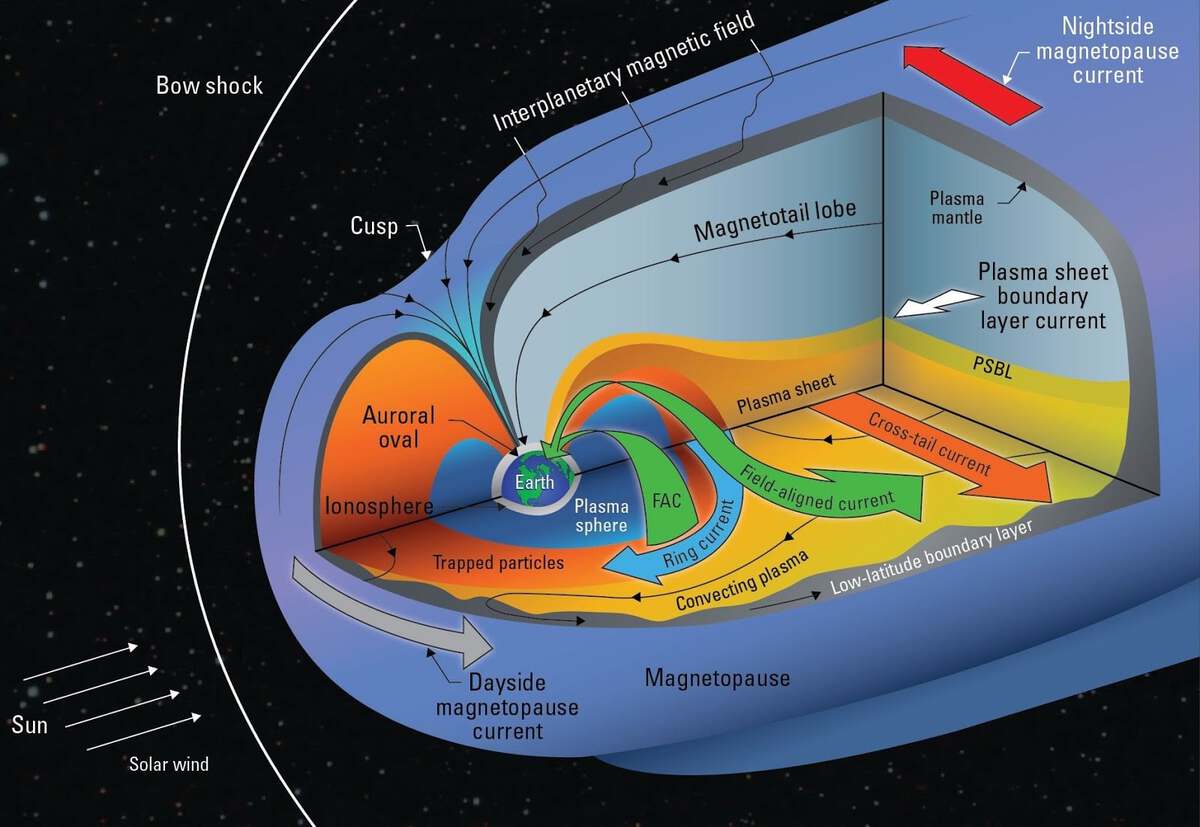
Geomagnetic storms are caused by the interaction of solar wind with Earth's magnetic field. The resulting disturbances in the geomagnetic field can wreak havoc on GPS systems, satellite communication, electric power transmission, and more. These disturbances are measured by the Disturbance Storm-Time Index, or Dst.
In the MagNet: Model the Geomagnetic Field competition, your task is to forecast Dst in real-time to help satellite operators, power grid operators, and users of magnetic navigation systems prepare for magnetic disturbances.
The primary input data for the challenge is provided by sensor data from two satellites, NASA's ACE and NOAA's DSCOVR. This space weather data includes sensor readings related to both the interplanetary magnetic field and plasma from solar wind.
Long Short Term Memory networks or LSTMs are a special kind of recurrent neural network especially suited to time series data. In this benchmark solution tutorial, we will show you how to implement a first-pass LSTM model for predicting Dst.
Specifically, we'll cover how to:
- load the data
- create features using the timedelta index
- generate batches of 32-length sequences for training
- train an LSTM model in Keras
- prepare
predict.pyfor code submission to the competition
Let's get started!
Getting Set Up
First, we'll import the basic tools we'll need to load our data and do some exploration.
from pathlib import Path

import matplotlib.pyplot as plt
import numpy as np
import pandas as pd

%load_ext nb_black
%matplotlib inline
Now we can read in our data. You can find everything you need on the data download page.
We're provided three datasets that could potentially be used as inputs:
solar_wind.csvsatellite_position.csvsunspots.csv
For now, we're going to ignore satellite_position.csv. This data could be useful because it describes the position of the satellite in relation to the Earth when the solar wind data was recorded. Feel free to experiment with using satellite positions as features in your model!
For the purposes of this tutorial, we're going to focus on the solar_wind and sunspot data. We'll also load up our labels, dst_labels.csv.
After reading in each csv, we're going to convert the timedelta columns to an actual timedelta object using pd.to_timdelta. That way we can take advantage of its convenient API.
Finally, we're going to set the indices of each dataframe to a multi-index composed of period and timedelta so that it's easier to join our dataframes.
DATA_PATH = Path("../data/final/public/")

dst = pd.read_csv(DATA_PATH / "dst_labels.csv")
dst.timedelta = pd.to_timedelta(dst.timedelta)
dst.set_index(["period", "timedelta"], inplace=True)

sunspots = pd.read_csv(DATA_PATH / "sunspots.csv")
sunspots.timedelta = pd.to_timedelta(sunspots.timedelta)
sunspots.set_index(["period", "timedelta"], inplace=True)

solar_wind = pd.read_csv(DATA_PATH / "solar_wind.csv")
solar_wind.timedelta = pd.to_timedelta(solar_wind.timedelta)
solar_wind.set_index(["period", "timedelta"], inplace=True)
Data Exploration
Let's start by looking at our label, dst. We have hourly values split into three periods - let's inspect the distribution of dst values across those periods.
print("Dst shape: ", dst.shape)
dst.head()
dst.groupby("period").describe()
We have nearly 140,000 observations of hourly dst data, representing over 15 years. There are almost twice as many observations in either the train_b or train_c periods than there are train_a. It also seems train_a represents a more intense period, given that it has a lower mean and higher standard deviation. Also note that most of the values are negative.
A very strong magnetic field disturbance has a large Dst value, measured in nano-Teslas (nT). Because these disturbances are usually flowing towards the Earth, the values are negative. Sometimes Dst can be highly positive. During calm conditions, Dst values are situated at or just below 0.
We can visualize the difference between the periods by plotting the distributions.
fig, ax = plt.subplots()
colors = ["r", "b", "y"]
for i, period in enumerate(dst.groupby("period")):
    period_name, df = period
    ax.hist(df, alpha=0.5, color=colors[i], bins=100, label=period_name)
plt.legend()
plt.title("Distribution of Dst across Periods")
plt.show()
Indeed, we can see that train_c is the most intense of the periods, followed by train_b. Let's keep this difference in distribution in mind when it comes to splitting the data.
For now, we can move on to exploring our features. The primary set of input data comes from the solar wind sensor readings gathered from the ACE and DSCOVR satellites. These measure characteristics of the interplanetary magnetic field (IMF) and plasma from solar wind.
For a complete description of the variables and what they represent, check out the competition Problem Description page.
Let's take a look:
print("Solar wind shape: ", solar_wind.shape)
solar_wind.head()
print("Sunspot shape: ", sunspots.shape)
sunspots.head()
We can see that we're mostly working with floats, except for the solar wind source column which tells us which of the two satellites recorded the data. We also see that the size of the solar_wind data is fairly large, close to 8.4 million rows. That makes sense, given we're working with minutely values.
On the other hand, we only have 192 observations of monthly sunspot data. When it comes to feature generation, we should think about the best ways to combine these features given their different frequencies.
Now let's look at the distribution of values across periods. We know that the distribution of dst is quite different, and we expect a similar pattern here.
solar_wind.groupby("period").describe().T
sunspots.groupby("period").describe().T
No surprise here. The mean and standard deviation of values in train_a is generally more intense than in the other two periods.
We also notice that our values exist across very different scales. For instance, temperature values are quite high - reaching into the hundreds of thousands Kelvin. Meanwhile, IMF readings are fairly small values, and usually negative. One of the best practices when training deep learning models is scaling your features; we'll definitely want to think about that later on.
Let's do a few visualizations before we move onto feature generation. First, we'll just plot the first 1,000 rows for some of our time series data to get a sense of its shape. Instead of plotting all of our features, let's just choose a few IMF features and a few plasma features.
def show_raw_visualization(data):
    fig, axes = plt.subplots(nrows=3, ncols=2, figsize=(15, 15), dpi=80)
    for i, key in enumerate(data.columns):
        t_data = data[key]
        ax = t_data.plot(
            ax=axes[i // 2, i % 2],
            title=f"{key.capitalize()}",
            rot=25,
        )

    fig.subplots_adjust(hspace=0.8)
    plt.tight_layout()


cols_to_plot = ["bx_gse", "bx_gsm", "bt", "density", "speed", "temperature"]
show_raw_visualization(solar_wind[cols_to_plot].iloc[:1000])
The first thing to notice is there are data gaps that we'll have to contend with. Let's count those:
solar_wind.isna().sum()
The proportion varies by feature, but every one will require some kind of imputation. Turns out sensor readings from space aren't always reliable - instruments are subject to all kinds of nasty space weather. It's up to us to figure out a sensible way of dealing with these missing values.
Another observation is that the IMF features bx_gsm and bx_gse are closely related. This could present multicollinearity issues if both are present in our model. As our last exploratory step, let's plot a correlation matrix to find other relationships between our features.
corr = solar_wind.join(sunspots).join(dst).fillna(method="ffill").corr()

plt.figure(figsize=(10, 5))
plt.matshow(corr, fignum=1)
plt.xticks(range(corr.shape[1]), corr.columns, fontsize=14, rotation=90)
plt.gca().xaxis.tick_bottom()
plt.yticks(range(corr.shape[1]), corr.columns, fontsize=14)


cb = plt.colorbar()
cb.ax.tick_params(labelsize=14)
plt.title("Feature Correlation Heatmap", fontsize=16)
plt.show()
Interesting! The plasma related features like speed and temperature look to be strongly anti-correlated with Dst. The IMF feature bt also exhibits strong anti-correlation.
As we suspected, the gsm and gse variables are strongly correlated. We probably want to leave some of those out.
With this information in hand, let's move onto feature generation.
Feature Generation
Before we get too far, let's first set seeds to make sure that all of our work is reproducible. We'll be using Keras, which makes use of both TensorFlow and numpy on the backend, so we'll be setting a seed for both.
from numpy.random import seed
from tensorflow.random import set_seed

seed(2020)
set_seed(2021)
Great! Now let's think about our feature processing pipeline. Let's recap what we've learned from data exploration:
- features exist across different scales
- features are provided at different frequencies
- certain IMF features are highly correlated
- there are many missing values
For the purposes of this tutorial, we'll address each of these issues using basic solutions. For your own implementations, you should get creative!
1. Features exist across different scales
We'll fix this using the StandardScaler from scikit-learn. It's a pretty standard affair - it'll help us subtract the mean and divide by the standard deviation for each feature. What's nice about it is that it'll save the parameters used for scaling so that we can re-use it later during prediction. You could also experiment with using the MinMaxScaler or other scaling methods instead.
2. Features are provided at different frequencies
One easy way to fix this is to aggregate values to the same frequency. Since our dst values are provided hourly, we'll aggregate solar_wind data to the hour. The timedelta API will make that really easy for us to group by the hour. We'll take both the mean and std of each value for each hour. This would be a great place to experiment with different frequencies and aggregations to try and get the best performance out of your model.
3. Certain IMF features are highly correlated
We'll solve this by taking a subset of the data. Let's use the plasma variables temperature, speed, and density, as well as the IMF feature bt. Since we saw that gse and gsm variables were highly correlated, let's only take the gse variables. This is a first pass at subsetting the variables - you may want to take a more principled approach in your implementation.
4. There are many missing values
We've already decided to aggregate our minutely solar wind data to an hourly frequency. That'll help with some of the missing values. For the remaining, there are a few different methods we could try. We want something that will be effective that will also work in a real-time environment. For simplicity, we're going to interpolate between missing values using df.interpolate(). Again, this is another great place for experimentation! You could impute using the mean or median, or you might even think about developing another model to estimate the missing values.
Finally, we have our monthly sunspot numbers. These aren't really "missing" - they're just provided at a coarser frequency. We'll fix that by using the forward fill or ffill method of imputation so that the correct monthly number is assigned to each row.
from sklearn.preprocessing import StandardScaler

# subset of solar wind features to use for modeling
SOLAR_WIND_FEATURES = [
    "bt",
    "temperature",
    "bx_gse",
    "by_gse",
    "bz_gse",
    "speed",
    "density",
]

# all of the features we'll use, including sunspot numbers
XCOLS = (
    [col + "_mean" for col in SOLAR_WIND_FEATURES]
    + [col + "_std" for col in SOLAR_WIND_FEATURES]
    + ["smoothed_ssn"]
)


def impute_features(feature_df):
    """Imputes data using the following methods:
    - `smoothed_ssn`: forward fill
    - `solar_wind`: interpolation
    """
    # forward fill sunspot data for the rest of the month
    feature_df.smoothed_ssn = feature_df.smoothed_ssn.fillna(method="ffill")
    # interpolate between missing solar wind values
    feature_df = feature_df.interpolate()
    return feature_df


def aggregate_hourly(feature_df, aggs=["mean", "std"]):
    """Aggregates features to the floor of each hour using mean and standard deviation.
    e.g. All values from "11:00:00" to "11:59:00" will be aggregated to "11:00:00".
    """
    # group by the floor of each hour use timedelta index
    agged = feature_df.groupby(
        ["period", feature_df.index.get_level_values(1).floor("H")]
    ).agg(aggs)
    # flatten hierachical column index
    agged.columns = ["_".join(x) for x in agged.columns]
    return agged


def preprocess_features(solar_wind, sunspots, scaler=None, subset=None):
    """
    Preprocessing steps:
        - Subset the data
        - Aggregate hourly
        - Join solar wind and sunspot data
        - Scale using standard scaler
        - Impute missing values
    """
    # select features we want to use
    if subset:
        solar_wind = solar_wind[subset]

    # aggregate solar wind data and join with sunspots
    hourly_features = aggregate_hourly(solar_wind).join(sunspots)

    # subtract mean and divide by standard deviation
    if scaler is None:
        scaler = StandardScaler()
        scaler.fit(hourly_features)

    normalized = pd.DataFrame(
        scaler.transform(hourly_features),
        index=hourly_features.index,
        columns=hourly_features.columns,
    )

    # impute missing values
    imputed = impute_features(normalized)

    # we want to return the scaler object as well to use later during prediction
    return imputed, scaler
Now let's apply our pipeline and see what your new data look like.
features, scaler = preprocess_features(solar_wind, sunspots, subset=SOLAR_WIND_FEATURES)
print(features.shape)
features.head()
# check to make sure missing values are filled
assert (features.isna().sum() == 0).all()
Our final feature set is composed of 15 features - the mean and standard deviation of seven solar_wind features, along with smoothed_ssn. We've also saved our scaler object. We'll serialize this later along with our model so that it can be used to preprocess features during prediction.
Before we start modeling, we also have to reshape our label, dst. Remember that we have to predict both t0, the current timestep, and t+1, an hour ahead. We'll train our LSTM to do multi-step prediction by providing it both steps. To do that, we just add another column called t1 that is dst shifted by 1. We'll also renamed our dst column to t0 for consistency.
YCOLS = ["t0", "t1"]


def process_labels(dst):
    y = dst.copy()
    y["t0"] = y.groupby("period").dst.shift(-1)
    y["t1"] = y.groupby("period").dst.shift(-2)
    return y[YCOLS]


labels = process_labels(dst)
labels.head()
Et voilà! Now we have our features and our labels. Let's join them together into one data df so that it's easier to keep the appropriate rows together when splitting into our train, test, and validation sets.
data = labels.join(features)
data.head()
Splitting the Data
We want to split our data into three datasets. As you might have guessed, the train set will be used for training. We'll also pass a validation set to keras as it's training to monitor the modeling fitting over epochs. Finally, we'll use a test set to evaluate our model for over or under fitting before we submit to the competition.
We have two atypical concerns to consider when splitting this dataset:
First, we're dealing with timeseries data. Observations in a time series are not indepedent, so we cannot randomly assign observations across our datasets. We also don't want to "cheat" by leaking future information into our training data. In the real-world, we will never be able to train on data from the future, so we should emulate those same contraints here.
Secondly, we have three non-contiguous periods, meaning we have gaps in our data. We don't know how long each gap is or in what order each period occured. We also know that the three periods are differently distributed. That suggests that observations from each period should be included in our train set, instead of reserving one wholesale as our test or validation set.
To solve these problems, we'll hold out the last 6,000 rows from each period for our test set, and reserve last 3,000 before that for our validation set. The remaining rows will be used in the training set.
def get_train_test_val(data, test_per_period, val_per_period):
    """Splits data across periods into train, test, and validation"""
    # assign the last `test_per_period` rows from each period to test
    test = data.groupby("period").tail(test_per_period)
    interim = data[~data.index.isin(test.index)]
    # assign the last `val_per_period` from the remaining rows to validation
    val = interim.groupby("period").tail(val_per_period)
    # the remaining rows are assigned to train
    train = interim[~interim.index.isin(val.index)]
    return train, test, val


train, test, val = get_train_test_val(data, test_per_period=6_000, val_per_period=3_000)
We can visualize our splits by plotting a horizontal barchart depicting the counts across periods.
ind = [0, 1, 2]
names = ["train_a", "train_b", "train_c"]
width = 0.75
train_cnts = [len(df) for _, df in train.groupby("period")]
val_cnts = [len(df) for _, df in val.groupby("period")]
test_cnts = [len(df) for _, df in test.groupby("period")]

p1 = plt.barh(ind, train_cnts, width)
p2 = plt.barh(ind, val_cnts, width, left=train_cnts)
p3 = plt.barh(ind, test_cnts, width, left=np.add(val_cnts, train_cnts).tolist())

plt.yticks(ind, names)
plt.ylabel("Period")
plt.xlabel("Hourly Timesteps")
plt.title("Train/Validation/Test Splits over Periods", fontsize=16)
plt.legend(["Train", "Validation", "Test"])
Let's do a final visual inspection of each of our datasets before we begin building our model.
print(train.shape)
train.head()
print(test.shape)
test.head()
print(val.shape)
val.head()
Building our Model
Now we can get started with model building!
The first thing we have to do is separate our data into sequences and batches for modeling. We have to decide on:
timesteps: this determines the sequence length, ie. how many timesteps in the past to use to predict each step at t0 and t1. Our data is aggregated hourly, so timesteps is equal to the number of hours we want to use for each prediction.batch_size: this determines the number of samples to work through before a model's parameters are updated.
For this tutorial, we'll choose fairly standard numbers of 32 timesteps per sequence and 32 sequences per batch. These numbers will likely have a large impact on your model, so feel free to experiment.
Now we need to use these numbers to separate our training data and labels into batches of sequences that will be fed into the model. Luckily, keras has just the tool with their timeseries_dataset_from_array function. According to the documentation:
If targets was passed, the dataset yields tuple (batch_of_sequences, batch_of_targets). If not, the dataset yields only batch_of_sequences.
This is exactly what we need! We can easily specify timesteps (referred to as sequence_length in the documentation) and batchsize to get a feature generator and a target generator that we can pass to model.fit(). For your implementation, you can experiment with different sequence_lengths along with sequence_stride (how many observations to skip between sequences) and sampling_rate (how many observations to sample per sequence).
There's one hiccup - we need to make sure that our sequences don't span across periods. To get around that, we'll iterate through our periods and generate a timeseries dataset for each one. Then we'll concatenate them at the end to rejoin our training set and validation set. And let's not forget - since we're only allowed to use feature data up until t-1, we'll need to realign our features and labels. We'll do that during our loop as well.
from keras import preprocessing


data_config = {
    "timesteps": 32,
    "batch_size": 32,
}


def timeseries_dataset_from_df(df, batch_size):
    dataset = None
    timesteps = data_config["timesteps"]

    # iterate through periods
    for _, period_df in df.groupby("period"):
        # realign features and labels so that first sequence of 32 is aligned with the 33rd target
        inputs = period_df[XCOLS][:-timesteps]
        outputs = period_df[YCOLS][timesteps:]

        period_ds = preprocessing.timeseries_dataset_from_array(
            inputs,
            outputs,
            timesteps,
            batch_size=batch_size,
        )

        if dataset is None:
            dataset = period_ds
        else:
            dataset = dataset.concatenate(period_ds)

    return dataset


train_ds = timeseries_dataset_from_df(train, data_config["batch_size"])
val_ds = timeseries_dataset_from_df(val, data_config["batch_size"])

print(f"Number of train batches: {len(train_ds)}")
print(f"Number of val batches: {len(val_ds)}")
Designing an LSTM
Finally, we need to design our LSTM network. We're going to build a simple sequential model with one hidden LSTM layer and one output later with 2 output values (t0 and t1). You can experiment by making your model deep (many layers) or wide (adding more neurons).
There are many hyperparameters that we can tune. We'll concentrate on a few here:
n_epochs: This determines the number of complete passes your model takes through the training data. For this tutorial, we'll choose 20 epochs. You'll want to monitor your rate of convergence to tune this number.n_neurons: The number of hidden nodes. Usually increases by powers of 2. We'll use 512.dropout: This regularizes by randomly "ignoring" a dropout fraction of a layer's neurons during each pass through the network during training, so that no particular neuron overfits its input. We'll start with a value of 0.4.stateful: This determines whether the model keeps track of the historical data that its seen within each batch. Since each sample within a batch encodes the entire sequence we care about, we can set this toFalse.
Tuning these values will impact how fast your model learns, whether it converges, and affect over/under fitting. Play around to see what works best.
After instantiating the model with these hyperparameters, we'll compile it with mean_squared_error as our loss function and adam as our optimizer. We'll have to remember to take the square root of our loss to get our competition metric, root_mean_squared_error.
from keras.layers import Dense, LSTM
from keras.models import Sequential

# define our model
model_config = {"n_epochs": 20, "n_neurons": 512, "dropout": 0.4, "stateful": False}

model = Sequential()
model.add(
    LSTM(
        model_config["n_neurons"],
        # usually set to (`batch_size`, `sequence_length`, `n_features`)
        # setting the batch size to None allows for variable length batches
        batch_input_shape=(None, data_config["timesteps"], len(XCOLS)),
        stateful=model_config["stateful"],
        dropout=model_config["dropout"],
    )
)
model.add(Dense(len(YCOLS)))
model.compile(
    loss="mean_squared_error",
    optimizer="adam",
)

model.summary()
Train Model
Now let's get to training! All we have to do is call model.fit() with our timeseries_dataset, batch_size, and epochs. We'll also set verbose to 0 to keep things tidy. At home, you can set it to 1 to print out a nice progress bar and the training and validation loss after each epoch.
Finally, we'll also pass it our valdation timeseries_dataset so that we can calcuate our validation loss along with our training loss after each epoch.
history = model.fit(
    train_ds,
    batch_size=data_config["batch_size"],
    epochs=model_config["n_epochs"],
    verbose=0,
    shuffle=False,
    validation_data=val_ds,
)
Evaluation
Huzzah! Our model finished training. We can plot the convergence by using our history object.
for name, values in history.history.items():
    plt.plot(values)
It looks like it was just starting to level out. On our next iteration, we could let it train for longer or try to adjust the hyperparemeters to get better convergence. Let' see how we did on our test set.
test_ds = timeseries_dataset_from_df(test, data_config["batch_size"])
mse = model.evaluate(test_ds)
print(f"Test RMSE: {mse**0.5:.2f}")
Since our metric is RMSE, we have to remember to take the square root. Looks like we ended up with a test RMSE of 14.24. Not bad! Let's prepare our code submission to see how we did on the competition test set.
Preparing for submission
First, we have to serialize everything we'll need for prediction (serialization just means convert to bytes so that we can store it on disk). That includes our StandardScaler, some of our configurations we used during preprocessing, and last but not least our model.
Keras provides a handy model.save() method for serializing models. We'll pickle our scaler and save our config to json.
import json
import pickle

model.save("model")

with open("scaler.pck", "wb") as f:
    pickle.dump(scaler, f)

data_config["solar_wind_subset"] = SOLAR_WIND_FEATURES
print(data_config)
with open("config.json", "w") as f:
    json.dump(data_config, f)
Finally, we have to prepare our predict.py file. This pulls together everything we need from our preprocessing pipeline down to prediction. We'll also have to load in any pieces that we serialized.
The following cell includes everything that we would write in predict.py.
Most crucially, it defines predict_dst. This is the function that that the code execution environment will call to get your predictions for t0 and t1 for any observations. In it, we'll process the data that we're passed and then call model.predict().
We'll also implement a simple safeguard to detect infinite or null predictions. If we return infinite or null values for t0 or t1, our submission will be automatically canceled. To avoid that, we'll return the mean dst of -12 when we detect any unexpected values. In reality, you'll want to debug your solution or implement a more sophisticated safeguard.
Check out the run time repo and code submission format page for details and how to put your code submission together.
import json
import pickle
from typing import Tuple

import keras
import numpy as np
import pandas as pd

# Load in serialized model, config, and scaler
model = keras.models.load_model("model")

with open("config.json", "r") as f:
    CONFIG = json.load(f)

with open("scaler.pck", "rb") as f:
    scaler = pickle.load(f)

# Set global variables
TIMESTEPS = CONFIG["timesteps"]
SOLAR_WIND_FEATURES = [
    "bt",
    "temperature",
    "bx_gse",
    "by_gse",
    "bz_gse",
    "speed",
    "density",
]
XCOLS = (
    [col + "_mean" for col in SOLAR_WIND_FEATURES]
    + [col + "_std" for col in SOLAR_WIND_FEATURES]
    + ["smoothed_ssn"]
)


# Define functions for preprocessing
def impute_features(feature_df):
    """Imputes data using the following methods:
    - `smoothed_ssn`: forward fill
    - `solar_wind`: interpolation
    """
    # forward fill sunspot data for the rest of the month
    feature_df.smoothed_ssn = feature_df.smoothed_ssn.fillna(method="ffill")
    # interpolate between missing solar wind values
    feature_df = feature_df.interpolate()
    return feature_df


def aggregate_hourly(feature_df, aggs=["mean", "std"]):
    """Aggregates features to the floor of each hour using mean and standard deviation.
    e.g. All values from "11:00:00" to "11:59:00" will be aggregated to "11:00:00".
    """
    # group by the floor of each hour use timedelta index
    agged = feature_df.groupby([feature_df.index.floor("H")]).agg(aggs)

    # flatten hierachical column index
    agged.columns = ["_".join(x) for x in agged.columns]
    return agged


def preprocess_features(solar_wind, sunspots, scaler=None, subset=None):
    """
    Preprocessing steps:
        - Subset the data
        - Aggregate hourly
        - Join solar wind and sunspot data
        - Scale using standard scaler
        - Impute missing values
    """
    # select features we want to use
    if subset:
        solar_wind = solar_wind[subset]

    # aggregate solar wind data and join with sunspots
    hourly_features = aggregate_hourly(solar_wind).join(sunspots)

    # subtract mean and divide by standard deviation
    if scaler is None:
        scaler = StandardScaler()
        scaler.fit(hourly_features)

    normalized = pd.DataFrame(
        scaler.transform(hourly_features),
        index=hourly_features.index,
        columns=hourly_features.columns,
    )

    # impute missing values
    imputed = impute_features(normalized)

    # we want to return the scaler object as well to use later during prediction
    return imputed, scaler


# THIS MUST BE DEFINED FOR YOUR SUBMISSION TO RUN
def predict_dst(
    solar_wind_7d: pd.DataFrame,
    satellite_positions_7d: pd.DataFrame,
    latest_sunspot_number: float,
) -> Tuple[float, float]:
    """
    Take all of the data up until time t-1, and then make predictions for
    times t and t+1.
    Parameters
    ----------
    solar_wind_7d: pd.DataFrame
        The last 7 days of satellite data up until (t - 1) minutes [exclusive of t]
    satellite_positions_7d: pd.DataFrame
        The last 7 days of satellite position data up until the present time [inclusive of t]
    latest_sunspot_number: float
        The latest monthly sunspot number (SSN) to be available
    Returns
    -------
    predictions : Tuple[float, float]
        A tuple of two predictions, for (t and t + 1 hour) respectively; these should
        be between -2,000 and 500.
    """
    # Re-format data to fit into our pipeline
    sunspots = pd.DataFrame(index=solar_wind_7d.index, columns=["smoothed_ssn"])
    sunspots["smoothed_ssn"] = latest_sunspot_number

    # Process our features and grab last 32 (timesteps) hours
    features, s = preprocess_features(
        solar_wind_7d, sunspots, scaler=scaler, subset=SOLAR_WIND_FEATURES
    )
    model_input = features[-TIMESTEPS:][XCOLS].values.reshape(
        (1, TIMESTEPS, features.shape[1])
    )

    # Make a prediction
    prediction_at_t0, prediction_at_t1 = model.predict(model_input)[0]

    # Optional check for unexpected values
    if not np.isfinite(prediction_at_t0):
        prediction_at_t0 = -12
    if not np.isfinite(prediction_at_t1):
        prediction_at_t1 = -12

    return prediction_at_t0, prediction_at_t1
We can zip this file up along with our serialized model and other pieces into a file called submission.zip.
Protip: In the noaa-runtime directory, you can put all of these files into /benchmark. Running make pack-benchmark will create a submission.zip in the /submission directory.
Now we can head over to the submissions page to submit our code.

Hooray! We got an RMSE of 16.3293. That's not a bad start, but now it's up to you to improve on it.
We hope this benchmark solution provided a helpful framework for exploring the solar wind data, designing an LSTM to predict Dst, and creating a code submission. We can't wait to see what else you come up with!
Head over to the MagNet: Model the Geomagnetic Field for more details on the competition. You can also check out the forum. Happy modeling!

