 A chimp next to the Zooniverse logo, the organization behind the crowd-sourced labels used in this competition.
Most of us don't get the chance to stroll around the jungle, gazing upon its Fantastic Beasts in awe. But thanks to motion and heat triggered camera traps, the jungle can now come to us. Camera traps enable researchers to observe the most sensitive habitats with minimal impact. Once set, camera traps can passively monitor a site, collecting many hours of footage.
However, annotating the footage collected by camera traps can be quite time-consuming. Even expert researchers must spend hundreds of hours doing simple species annoation — time that they'd rather be spending exploring the deeper questions realted to the wildlife ecology of the seat of life on Earth.
In our brand new competition, we're helping make it easier for research teams to study camera trap footage by predicting the species present in a given video. Automated video species tagging could save many human hours of annotation, allowing researchers to focus on higher-level research and conservation efforts.
In this post, we'll walk through a very simple first pass model for species classification in camera trap footage. Video data can be intimidating, but this post will show how to load the data, make some predictions, and then submit those predictions to the competition.
Okay, to get things rolling, let's load up some basic tools of the trade.
%matplotlib inline

import os

# let's not pollute this blog post with warnings
from warnings import filterwarnings

filterwarnings("ignore")

import keras
import numpy as np
import pandas as pd
import skvideo.io as skv
from tqdm import tqdm
Loading the data
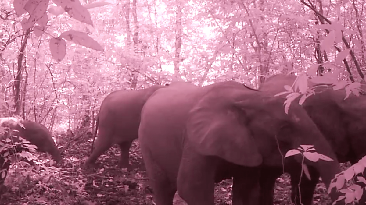 Camera trap footage of some elephants strolling along, taken from the dataset!
On the data download page, we provide a couple of datasets to get started:
- Camera trap footage: we have a few hundred thousand clips from camera traps around Africa. These are our main model inputs. The raw data is over 1TB, so we've created extremely downsampled versions of the dataset to facilitate faster prototyping. There is the micro version of the data, which is about 3.5 GB, and the nano version, which is about 1.5 GB. All versions are hosted as direct downloads and as well as torrent files. For this benchmark we'll use the nano data.
- Crowd-sourced species labels for camera trap training set: generated by thousands of citizen scientists at Chimp&See. These are our labels. Each row is indexed by a video filename and each column corresponds to a species that may or may not be present in the video as indicated by a 1 or 0 respectively.
- Submission format: This gives us the filenames and columns of our submission prediction, filled with all zeros as a baseline. The filenames should be used to index into the video directory (e.g., nano) to generate test predictions.
One of the fun things about this challenge is that multiple species may be present in a given video, making this a multilabel classification challenge. That's why each video has so many columns associated with it.
Let's check out some of the training labels!
# load the data
labelpath = os.path.join("..", "data", "final", "train_labels.csv")
train_labels = pd.read_csv(labelpath, index_col="filename")
train_labels.head()
# How many training videos do we have, and what species are present?
train_labels.info()
There are a lot of cool species in these videos! Also, no NaNs in sight. It's going to be a good day.
# How many of each species?
train_labels.sum(axis=0).sort_values(ascending=False)
Looking through the data, we see that most of the videos are blank, meaning there is no species present. This could mean that the traps are triggered too easily, but in any case it's useful to keep in mind for modeling.
On the upside, there are thousands of chimps, a bunch of elephants, and tons of DrivenData's new official mascot: the duiker.
# How many videos have more than one species present?
(train_labels.sum(axis=1) > 1).sum()
Ok, not too many in the training data, but still woth considering since we have the power of deep learning at our fingertips.
We're almost ready to turn to the prediction task, but first a word on working with the videos themselves.
- We built a custom Dataset class for handling batch generation and storing predictions. Working with video can be annoying to say the least. In order to facilitate faster model prototyping, we have written a
Datasetclass that can be used by the keras.fit_generator()method to serve batches of training data. It uses thefilenames in the data csvs to index into the video directory. It also stores useful information about the dataset, such as number of samples, size of the videos, and even validation splits!
The class — which is available if you download these two files and placing them in the same directory as your notebook — has only been tested for use with the nano and micro versions of the datasets. If you try to use it with the raw version, there will likely be some edits neccessary since the videos aren't square.
The dataset class also assumes that the datapath directory contains
- a directoy
dataset_typenamednano,micro, orraw. train_labels.csvsubmission_format.csv
We're going to store the instance of he dataset as data, so data.anything is using the class. Feel free to play around with this and build it out more, or abandon it completely!
# import the custom data handler
from primatrix_dataset_utils import Dataset
datapath = os.path.join("..", "data", "final")
data = Dataset(datapath=datapath, reduce_frames=True, batch_size=32, test=False)
# confirm number of classes
data.num_classes
# reduced frame count for faster processing
data.num_frames
# check our batch size
data.batch_size
# number of training samples
data.num_samples
We're not going to train on all of those samples. We'll instead use around 30,000
The Error Metric - AggregatedLogLoss
Performance is evaluated according to an aggregated log loss. This is similar to the binary log loss, but to acccount for the possibility of multiple labels treats each column as its own, independent binary log loss and sums the results for all labels.
To see how this metric manifests in our Keras model below, note the sigmoid activation of the final layer of the network, as well as the binary_crossentropy loss function specified in model.compile(). Keras infers the multilabel nature of the problem automatically by looking at the shape of the labels.
Building a Model
 What can't it do?
There are many ways we could approach this modelling problem. One of the simplest might be to extract a frame from each video and train a basic image classifer on the result. Of course, animals may move in and out of frame making our chosen frame very important. The most sophisticated approaches might use the raw video data as input to get the most out of every pixel. Here, we'll stick with something in between.
We're going to use keras (not PyTorch, sorry ;-)) to train a multilabel video classifier on the nano dataset, taking a downsampled version of the nano videos as input. Additionally, in the interest of training time, we're going to train our model on a subset of training data. However, we'll predict on the full set.
Our general workflow will be to:
- Build a model architecture
- Train for a couple epochs with validation
- Generate predctions for the entire test set.
First let's consider a couplw of key aspects of the model environment.
Model Environment
The goal of this benchmark is to provide a clear path from data download to prediction submission. In that spirit, we're going to train a simple model on a subset of the nano version of the camera trap footage.
Since we're processing video tensors, using a GPU will still provide substantial speedup. If using Amazon Web Services is an option for you, we reccomend
- Spinning up an EC2 instance with a GPU
- Installing FFMPEG to the instance for video processing
- Setting up your deep leanring environment with jupyter (we're going to use keras with a tensorflow backend)
- Creating an SSH tunnel so that you can access your gpu-powered Jupyter notebook from the comport of your own browser!
As always, make sure to avoid unneccessary charges by stopping your EC2 instance when not training or editing code!
GPU
First we check this AWS instance sees our GPU!
If the below doesn't work for you, here is a relatively painless guide to setting up your GPU and tensorflow on AWS Ubuntu 16.04.
%%bash
nvidia-smi
Great, now let's make sure our tensorflow backend is using the GPU using the following handy method.
from tensorflow.python.client import device_lib


def get_available_gpus():
    local_device_protos = device_lib.list_local_devices()
    return [x.name for x in local_device_protos if x.device_type == "GPU"]


print(f"Available GPUs:\t{get_available_gpus()}")
Alright! Now we're ready to go deep...
Build the Model
We're going to classify our data using a very simple version of of the Long-term Recurrent Convolutional Network deep learning architecture, also known as LRCN architecture:
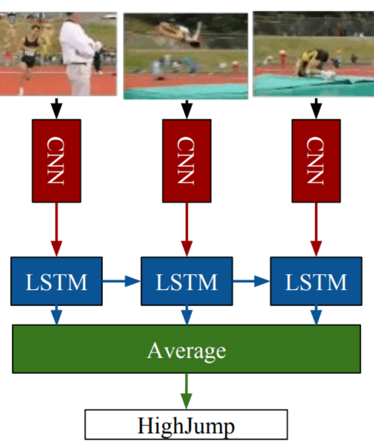
LRCNs extract features using convolutional layers and pass those as inputs to a Long short-term Memory network for classification.
We can use the built-in keras TimeDistributed wrapper to easily enable temporal convolutional processing of video tensors.
Let's import the keras objects we need.
from keras.models import Sequential
from keras.layers import TimeDistributed, Conv2D, MaxPooling2D, Flatten, Dropout, Dense
from keras.layers.recurrent import LSTM
Simple Keras LRCN
The model we build below is by no means optimized, but it's a start! The goal of this benchmark is to present one possible workflow from data download to competition submission.
# instantiate model
model = Sequential()

# add three time-distributed convolutional layers for feature extraction
model.add(
    TimeDistributed(
        Conv2D(64, (3, 3), activation="relu"),
        input_shape=(data.num_frames, data.width, data.height, 1),
    )
)
model.add(TimeDistributed(MaxPooling2D((2, 2), strides=(1, 1))))

model.add(TimeDistributed(Conv2D(128, (4, 4), activation="relu")))
model.add(TimeDistributed(MaxPooling2D((2, 2), strides=(2, 2))))

model.add(TimeDistributed(Conv2D(256, (4, 4), activation="relu")))
model.add(TimeDistributed(MaxPooling2D((2, 2), strides=(2, 2))))


# extract features and dropout
model.add(TimeDistributed(Flatten()))
model.add(Dropout(0.5))

# input to LSTM
model.add(LSTM(256, return_sequences=False, dropout=0.5))

# classifier with sigmoid activation for multilabel
model.add(Dense(data.num_classes, activation="sigmoid"))

# compile the model with binary_crossentropy loss for multilabel
model.compile(optimizer="rmsprop", loss="binary_crossentropy")

# look at the params before training
model.summary()
Train the Model
Alright, let's train this net! Notice below that we've commented out parameters that would allow training on the entire dataset. We've also set epochs=2 because well, we don't have all day over here – training a winning model is your job!
# train the model with validation
model.fit_generator(
    data.batches(),
    steps_per_epoch=500,  # data.num_batches to train on full set
    epochs=2,
    validation_data=data.val_batches(),
    validation_steps=30,  # data.num_val_batches to validate on full set
)
Save the Model
Deep learning networks can take a long time to train, so it's always a good idea to save the learned parameters!
# save model
benchmark_model_name = "benchmark-model.h5"
model.save(benchmark_model_name)
Time to Predict and Submit
And now we make our predictions! We will load the saved model and test on every video in the index of the submission_format.csv. As before, the batch generation is handled by our custom Dataset class, which is available for you to download.
# load model
from keras.models import load_model

trained_model = load_model(benchmark_model_name)
# generate predictions
for batch_num in tqdm(range(data.num_test_batches), total=data.num_test_batches):
    # make predictions on batch
    results = trained_model.predict_proba(
        next(data.test_batches()), batch_size=data.batch_size, verbose=0
    )

    # update submission format dataframe stored in dataset object
    data.update_predictions(results)
Save Predictions
All we have to do now is save our predictions and make a submission. Just to confirm that we're following the submission format, let's look at the first few rows:
# save results!
data.predictions.to_csv(os.path.join(data.datapath, "predictions.csv"))
!head -n 5 ../data/final/predictions.csv
Looks good, now we can submit it to the competition.
Submit to Leaderboard

Woohoo! It's a start! And that's exactly what we intend with these benchmarks. We're sure you'll be able to top this model in no time, and we can't wait to see what you come up with.
 Just don't be fooled by imposters!
